Customer Lifetime Value (CLV)

1. Project Overview

My starting point for this project is to frame two common business problems faced by the Google Merchandise Store and ecommerce businesses in general.

1.1 Frame the business problems

• What will customers spend in the next 90-days? (Regression)
• What is the probability that a customer will make a purchase in the next 90-days? (Classification)

In order to provide insights to these questions, we first need to :

1.2 Translate the raw data into meaningful visualizations and insights

• explore the dataset to extract meaningful trends, patterns and anomalies regarding customer behaviour
• visualize using plotly and plotnine
• create additional RMF (Recency, Monetary, Frequency) to unlock hidden insights

1.3 Use the insights to make future predictions

• train a machine learning regression model to etablish a BASELINE prediction of the $ customer spend in the next-90 days
• train a machine learning classification model to establish a BASELINE prediction of the likelihood of customer spend in the next-90 days

In practice we would adopt an iterative process, by trying a range of different models and choosing the one that presents the best compromise between training speed (cost), accuracy and explainability. The more complex the model the more accurate the results generally, but with a trade off in interpretability.

1.4 Communicate using an interactive dashboard

• present the findings of my analysis through an interactive dashboard
• share my findings through deployment of a Dash ecommerce customer analytics app

1.5 Move from insights to actionable outcomes

We can use these predictions to identify :

• Which customers have the highest spend probability in next 90-days?

target for new products similar to what they have purchased in the past

• Which customers have recently purchased (within 90 days) but are unlikely to buy (probability less than 30%)?

incentivize actions to increase probability
provide discounts, encourage referring a friend, nurture by letting them know what’s coming

• Missed opportunities: Big spenders that could be unlocked?

Send bundle offers encouraging volume purchases
Focus on missed opportunities

By adopting this approach ecommerce businesses can make informed decisions to improve customer satisfaction, increase sales, and enhance overall operational efficiency.

2. Customer Lifetime Value

Companies use this metric to gauge profitability and to identify which customers to focus on. In short, CLV is the estimated profit from the future relationship with a customer. There are many different approaches to modeling CLV.

2.1 Economic / cashflow approach

cashflow.JPG

Challenges with this approach:

• Lifetime value is great, but more important is a pre-defined period of time, for example the next 90-days

2.2 Machine learning approach

• Step 1: Subset a cohort
• Step 2: Temoral splitting - use future information to develop targets
• Step 3: Create RFM features (Recency, Frequency, Monetary)

3. Dataset, schema, packages

The dataset I will be analysing is the Google Analytics sample dataset for BigQuery.

The sample dataset contains obfuscated Google Analytics 360 data from the Google Merchandise Store, a real ecommerce store. The Google Merchandise Store sells Google branded merchandise. The data is typical of what you would see for an ecommerce website. It includes the following kinds of information:

• Traffic source data: information about where website visitors originate. This includes data about organic traffic, paid search traffic, display traffic, etc.
• Content data: information about the behavior of users on the site. This includes the URLs of pages that visitors look at, how they interact with content, etc.
• Transactional data: information about the transactions that occur on the Google Merchandise Store website.

The dataset covers the 366 day period 1 August 2016 to 1 August 2017.

3.1 Schema

Before diving into our analysis, it is good practice to explore the dataset schema.

If you take a close look at the schema you will see that the structure involves nested fields. It can be extremely cost-effective (both in terms of storage and in terms of query time) to use nested fields rather than flatten out all your data. Nested, repeated fields are very powerful, but the SQL required to query them looks a bit unfamiliar. So, it’s worth spending a little time with STRUCT, UNNEST and ARRAY_AGG.

Fields which are of type INTEGER or STRING can be accessed directly. However things a bit trickier as we go deeper into the structure.

totals for example is of Type RECORD and includes sub-variables. In order to access these we need to use dot notation:

totals.visits

Things get even trickier with fields of Type RECORD and Mode Repeated, for example hits. In order to access the subvariable hitNumber we need to use the UNNEST() function, give it an alias, and then we can use dot notation :

SELECT
    h.hitNumber
FROM
`bigquery-public-data.google_analytics_sample.ga_sessions_*`,
UNNEST(hits) AS h

We can go even deeper. To access hits.product.productRevenue we need to first UNNEST hits and then because product is also of Type RECORD and Mode Repeated we have to UNNEST(hits.product). Expanding on the above example :

SELECT
    h.hitNumber,
    p.productRevenue
FROM
`bigquery-public-data.google_analytics_sample.ga_sessions_*`,
UNNEST(hits) AS h,
UNNEST(hits.product) AS p

Google cloud have learnng resources to help you.

OK, now that I’ve gotten to know the dataset a bit better it’s time to dive into some exploratory analysis.

3.2 A Kind of Magic

magic.jpg

Jupyter notebooks (which i am using for this project) provide a convenient interactive computing environment for various programming languages, including Python. You might be aware of so called magic commands, denoted by a % or %% symbol. These are special commands that enhance the functionality and provide additional features within Jupyter notebooks. Here’s a brief summary of some commonly used magic commands:

Line Magic Commands (%):

• %run: Execute a Python script as if it were a program.
• %load: Load code into a cell from an external script.
• %pwd: Print the current working directory.
• %cd: Change the current working directory.
• %ls: List the contents of the current directory.
• %matplotlib: Enable interactive Matplotlib plots.

Cell Magic Commands (%%):

• %%time: Measure the time it takes for the code in the cell to run.
• %%html: Render the cell content as HTML.

Interactive Shell Commands:

• !: Run shell commands directly from a Jupyter cell.

3.3 Import packages and libraries

%load_ext google.cloud.bigquery 
from google.cloud import bigquery
import google.cloud.bigquery
from google.oauth2 import service_account

import pandas as pd
pd.set_option('display.max_columns', None)
import numpy as np
import pytimetk as tk
import plotly.express as px
import joblib 
from missingno import matrix # missing data

#!pip install plydata
import plydata.cat_tools as cat
import plotnine as pn
import pytimetk as tk
from xgboost import XGBClassifier, XGBRegressor
from sklearn.model_selection import GridSearchCV

pn.options.dpi = 300

4. Exploratory Data Analysis

4.1 Using %%bigquery to run SQL within Jupyter

The %%bigquery magic which allows you to run SQL queries on data held in BigQuery from the comfort of your own local Jupyter Notebook.

The data is separated into daily tables but you can use _* to access everything, and if you specify a name after %%big query, it will return a pandas DataFrame!

%%bigquery total_days
SELECT COUNT(DISTINCT date) AS number_days
FROM `bigquery-public-data.google_analytics_sample.ga_sessions_*`

total_days

	number_days
0	366

type(total_days)

pandas.core.frame.DataFrame

%%bigquery
SELECT COUNT(*)
FROM `bigquery-public-data.google_analytics_sample.ga_sessions_*`

	f0_
0	903653

Ok, so the dataset covers a period of 366 days and contains 903,653 rows. Let’s preview one day :

%%bigquery sample_day
SELECT *
FROM `bigquery-public-data.google_analytics_sample.ga_sessions_20170713`

sample_day

	visitorId	visitNumber	visitId	visitStartTime	date	totals	trafficSource	device	geoNetwork	customDimensions	hits	fullVisitorId	userId	clientId	channelGrouping	socialEngagementType
0	<NA>	2	1500008750	1500008750	20170713	{'visits': 1, 'hits': 1, 'pageviews': 1, 'time...	{'referralPath': None, 'campaign': '(not set)'...	{'browser': 'Firefox', 'browserVersion': 'not ...	{'continent': 'Americas', 'subContinent': 'Nor...	[{'index': 4, 'value': 'North America'}]	[{'hitNumber': 1, 'time': 0, 'hour': 22, 'minu...	137294517588272857	None	None	Direct	Not Socially Engaged
1	<NA>	1	1499957243	1499957243	20170713	{'visits': 1, 'hits': 1, 'pageviews': 1, 'time...	{'referralPath': None, 'campaign': '(not set)'...	{'browser': 'Chrome', 'browserVersion': 'not a...	{'continent': 'Americas', 'subContinent': 'Nor...	[{'index': 4, 'value': 'North America'}]	[{'hitNumber': 1, 'time': 0, 'hour': 7, 'minut...	4373106646092857768	None	None	Direct	Not Socially Engaged
2	<NA>	1	1499968083	1499968083	20170713	{'visits': 1, 'hits': 1, 'pageviews': 1, 'time...	{'referralPath': None, 'campaign': '(not set)'...	{'browser': 'Safari', 'browserVersion': 'not a...	{'continent': 'Americas', 'subContinent': 'Nor...	[{'index': 4, 'value': 'North America'}]	[{'hitNumber': 1, 'time': 0, 'hour': 10, 'minu...	160773093174680026	None	None	Direct	Not Socially Engaged
3	<NA>	2	1499952856	1499952856	20170713	{'visits': 1, 'hits': 1, 'pageviews': 1, 'time...	{'referralPath': None, 'campaign': '(not set)'...	{'browser': 'Chrome', 'browserVersion': 'not a...	{'continent': 'Americas', 'subContinent': 'Nor...	[{'index': 4, 'value': 'North America'}]	[{'hitNumber': 1, 'time': 0, 'hour': 6, 'minut...	1117853031731048699	None	None	Direct	Not Socially Engaged
4	<NA>	4	1499982847	1499982847	20170713	{'visits': 1, 'hits': 1, 'pageviews': 1, 'time...	{'referralPath': None, 'campaign': '(not set)'...	{'browser': 'Chrome', 'browserVersion': 'not a...	{'continent': 'Americas', 'subContinent': 'Nor...	[{'index': 4, 'value': 'North America'}]	[{'hitNumber': 1, 'time': 0, 'hour': 14, 'minu...	1319757127869798182	None	None	Display	Not Socially Engaged
...	...	...	...	...	...	...	...	...	...	...	...	...	...	...	...	...
2736	<NA>	1	1499986111	1499986111	20170713	{'visits': 1, 'hits': 73, 'pageviews': 57, 'ti...	{'referralPath': None, 'campaign': '(not set)'...	{'browser': 'Safari', 'browserVersion': 'not a...	{'continent': 'Americas', 'subContinent': 'Nor...	[{'index': 4, 'value': 'North America'}]	[{'hitNumber': 1, 'time': 0, 'hour': 15, 'minu...	4100305414080508541	None	None	Organic Search	Not Socially Engaged
2737	<NA>	5	1499969354	1499969354	20170713	{'visits': 1, 'hits': 86, 'pageviews': 57, 'ti...	{'referralPath': '/', 'campaign': '(not set)',...	{'browser': 'Chrome', 'browserVersion': 'not a...	{'continent': 'Americas', 'subContinent': 'Nor...	[{'index': 4, 'value': 'North America'}]	[{'hitNumber': 1, 'time': 0, 'hour': 11, 'minu...	806992249032686650	None	None	Referral	Not Socially Engaged
2738	<NA>	1	1499931174	1499931174	20170713	{'visits': 1, 'hits': 132, 'pageviews': 85, 't...	{'referralPath': None, 'campaign': '(not set)'...	{'browser': 'Safari', 'browserVersion': 'not a...	{'continent': 'Americas', 'subContinent': 'Nor...	[{'index': 4, 'value': 'North America'}]	[{'hitNumber': 1, 'time': 0, 'hour': 0, 'minut...	3917496719101325275	None	None	Direct	Not Socially Engaged
2739	<NA>	1	1499951313	1499951315	20170713	{'visits': 1, 'hits': 156, 'pageviews': 109, '...	{'referralPath': None, 'campaign': '(not set)'...	{'browser': 'Chrome', 'browserVersion': 'not a...	{'continent': 'Americas', 'subContinent': 'Nor...	[{'index': 4, 'value': 'North America'}]	[{'hitNumber': 2, 'time': 0, 'hour': 6, 'minut...	9417857471295131045	None	None	Direct	Not Socially Engaged
2740	<NA>	1	1499982367	1499982367	20170713	{'visits': 1, 'hits': 169, 'pageviews': 86, 't...	{'referralPath': '/intl/sr/yt/about/copyright/...	{'browser': 'Chrome', 'browserVersion': 'not a...	{'continent': 'Europe', 'subContinent': 'South...	[]	[{'hitNumber': 1, 'time': 0, 'hour': 14, 'minu...	0707769484819212214	None	None	Social	Not Socially Engaged

2741 rows × 16 columns

As previously discussed, a lot of nested fields to unravel.

sample_day.glimpse()

<class 'pandas.core.frame.DataFrame'>: 2741 rows of 16 columns
visitorId:             Int64             [<NA>, <NA>, <NA>, <NA>, <NA>,  ...
visitNumber:           Int64             [2, 1, 1, 2, 4, 1, 3, 2, 1, 1,  ...
visitId:               Int64             [1500008750, 1499957243, 149996 ...
visitStartTime:        Int64             [1500008750, 1499957243, 149996 ...
date:                  object            ['20170713', '20170713', '20170 ...
totals:                object            [{'visits': 1, 'hits': 1, 'page ...
trafficSource:         object            [{'referralPath': None, 'campai ...
device:                object            [{'browser': 'Firefox', 'browse ...
geoNetwork:            object            [{'continent': 'Americas', 'sub ...
customDimensions:      object            [array([{'index': 4, 'value': ' ...
hits:                  object            [array([{'hitNumber': 1, 'time' ...
fullVisitorId:         object            ['137294517588272857', '4373106 ...
userId:                object            [None, None, None, None, None,  ...
clientId:              object            [None, None, None, None, None,  ...
channelGrouping:       object            ['Direct', 'Direct', 'Direct',  ...
socialEngagementType:  object            ['Not Socially Engaged', 'Not S ...

4.2 Generate our master data for further analysis

%%bigquery google_merch_store

SELECT 
    fullVisitorId,
    date,    
    product.productQuantity AS quantity,
    product.v2ProductName AS product_name,
    product.productPrice / 1000000 AS price, 
    product.productQuantity * product.productPrice / 1000000 AS product_revenue,
    totals.totalTransactionRevenue / 1000000 AS total_transaction_revenue
FROM
    `bigquery-public-data.google_analytics_sample.ga_sessions_*`, 
    UNNEST (hits) AS hits, 
    UNNEST(hits.product) AS product
WHERE 
    hits.eCommerceAction.action_type = '6' # Completed purchase    
    AND product.productQuantity > 0
    AND product.productPrice > 0 
    AND totals.totalTransactionRevenue > 0 # This value is 1 for sessions with interaction events.
ORDER BY
    date

google_merch_store

	fullVisitorId	date	quantity	product_name	price	product_revenue	total_transaction_revenue
0	3213840074316400693	20160801	20	Color Changing Grip Pen	1.20	24.00	170.40
1	3213840074316400693	20160801	20	Kick Ball	1.59	31.80	170.40
2	3213840074316400693	20160801	20	Electronics Accessory Pouch	3.99	79.80	170.40
3	3213840074316400693	20160801	20	Badge Holder	1.59	31.80	170.40
4	2976178532750719771	20160801	4	Maze Pen	0.99	3.96	19.93
...	...	...	...	...	...	...	...
36741	8016003971239765913	20170801	2	Android Men's Short Sleeve Hero Tee White	6.80	13.60	131.96
36742	8016003971239765913	20170801	1	Women's Performance Full Zip Jacket Black	67.19	67.19	131.96
36743	8016003971239765913	20170801	1	Android Men's Engineer Short Sleeve Tee Charcoal	15.99	15.99	131.96
36744	8016003971239765913	20170801	1	Google Infant Short Sleeve Tee Red	13.59	13.59	131.96
36745	8016003971239765913	20170801	1	Android Infant Short Sleeve Tee Pewter	13.59	13.59	131.96

36746 rows × 7 columns

4.3 PyTimeTK

While the Python ecosystem offers tools like pandas, they sometimes can be verbose and not optimized for all operations, especially for complex time-based aggregations and visualizations. pytimetk significantly simplifies the process of time series manipulation and visualization. By leveraging the polars backend, you can experience speed improvements ranging from 3X to 3500X.

A usefuly feature is .glimpse() which does what it says on the tin :

google_merch_store.glimpse()

<class 'pandas.core.frame.DataFrame'>: 36746 rows of 7 columns
fullVisitorId:              object            ['3213840074316400693', '3 ...
date:                       object            ['20160801', '20160801', ' ...
quantity:                   Int64             [20, 20, 20, 20, 4, 1, 1,  ...
product_name:               object            ['Color Changing Grip Pen' ...
price:                      float64           [1.2, 1.59, 3.99, 1.59, 0. ...
product_revenue:            float64           [24.0, 31.8, 79.8, 31.8, 3 ...
total_transaction_revenue:  float64           [170.4, 170.4, 170.4, 170. ...

4.4 Custom profile function

This custom function aids the EDA process and is a pseeudo hybrid of pandas .info() and .describe() :

# Custom profiling function
def profile_data(data):
    """Panda Profiling Function

    Args:
        data (DataFrame): A data frame to profile

    Returns:
        DataFrame: A data frame with profiled data
    """
    return pd.concat(
        [
            pd.Series(data.dtypes, name = "Dtype"),
            # Counts
            pd.Series(data.count(), name = "Count"),
            pd.Series(data.isnull().sum(), name = "NA Count"),
            pd.Series(data.nunique(), name = "Count Unique"),
            # Stats
            pd.Series(data.min(), name = "Min"),
            pd.Series(data.max(), name = "Max"),
            pd.Series(data.mean(), name = "Mean"),
            pd.Series(data.median(), name = "Median"),
            pd.Series(data.mode().iloc[0], name = "Mode"),
        ],
        axis=1
    )

profile_data(google_merch_store)

	Dtype	Count	NA Count	Count Unique	Min	Max	Mean	Median	Mode
fullVisitorId	object	36746	0	9995	0000213131142648941	9998996003043230595	inf	4.512553e+18	1957458976293878100
date	object	36746	0	365	20160801	20170801	inf	2.017013e+07	20161212
quantity	Int64	36746	0	123	1	1000	6.423584	1.000000e+00	1
product_name	object	36746	0	490	1 oz Hand Sanitizer	YouTube Youth Short Sleeve Tee Red	NaN	NaN	Google Sunglasses
price	float64	36746	0	264	0.79	250.0	16.602405	1.329000e+01	13.59
product_revenue	float64	36746	0	2001	0.79	9495.0	45.727660	1.749000e+01	13.59
total_transaction_revenue	float64	36746	0	6199	1.2	47082.06	366.675515	1.022000e+02	23.99

So we can very quickly see that our dataset consists of 36,746 purchase transactions made by 9,995 unique customers and the common purchase was Google sunglasses.

Before we progress, we need to convert date from an object type to datetime:

# Convert the date column to datetime64 with nanosecond precision
google_merch_store['date'] = pd.to_datetime(google_merch_store['date'], format='%Y%m%d')

google_merch_store.glimpse()

<class 'pandas.core.frame.DataFrame'>: 36746 rows of 7 columns
fullVisitorId:              object            ['3213840074316400693', '3 ...
date:                       datetime64[ns]    [Timestamp('2016-08-01 00: ...
quantity:                   Int64             [20, 20, 20, 20, 4, 1, 1,  ...
product_name:               object            ['Color Changing Grip Pen' ...
price:                      float64           [1.2, 1.59, 3.99, 1.59, 0. ...
product_revenue:            float64           [24.0, 31.8, 79.8, 31.8, 3 ...
total_transaction_revenue:  float64           [170.4, 170.4, 170.4, 170. ...

5. Feature pre-processing

5.1.1 Subset a Cohort

# Show only the first transaction made by each unique customer
cust_first_purch = google_merch_store \
    .sort_values(['fullVisitorId', 'date']) \
    .groupby('fullVisitorId') \
    .first()

cust_first_purch

	date	quantity	product_name	price	product_revenue	total_transaction_revenue
fullVisitorId
0000213131142648941	2017-04-28	1	BLM Sweatshirt	33.59	33.59	39.59
0002871498069867123	2016-08-23	15	Google Metallic Notebook Set	5.99	89.85	97.35
0003450834640354121	2016-10-18	1	Google Laptop and Cell Phone Stickers	1.99	1.99	59.95
0003961110741104601	2017-05-21	1	YouTube Custom Decals	1.99	1.99	10.98
000435324061339869	2016-10-20	1	Google Men's Zip Hoodie	44.79	44.79	46.79
...	...	...	...	...	...	...
9991633376050115277	2017-02-17	1	BLM Sweatshirt	33.59	33.59	35.59
9994767073213036303	2016-08-09	3	Electronics Accessory Pouch	4.99	14.97	140.32
9997409246962677759	2016-12-08	1	Crunch Noise Dog Toy	3.99	3.99	40.36
9998597322098588317	2016-08-01	30	PaperMate Ink Joy Retractable Pen	1.25	37.50	102.20
9998996003043230595	2016-11-16	1	Google Vintage Henley Grey/Black	29.99	29.99	66.98

9995 rows × 6 columns

cust_first_purch['date'].min()

Timestamp('2016-08-01 00:00:00')

cust_first_purch['date'].max()

Timestamp('2017-08-01 00:00:00')

5.1.2 Visualize all purchases within cohort

# grab date values for our y axis, and price for our x axis
google_merch_store \
    .reset_index() \
    .set_index('date')[['price']]

	price
date
2016-08-01	1.20
2016-08-01	1.59
2016-08-01	3.99
2016-08-01	1.59
2016-08-01	0.99
...	...
2017-08-01	6.80
2017-08-01	67.19
2017-08-01	15.99
2017-08-01	13.59
2017-08-01	13.59

36746 rows × 1 columns

# Aggregate all customer revenue per month
google_merch_store\
    .reset_index() \
    .set_index('date')[['price']] \
    .resample(
        rule = "MS" # group by month
    ) \
    .sum()

	price
date
2016-08-01	68604.07
2016-09-01	44910.37
2016-10-01	45032.57
2016-11-01	48906.36
2016-12-01	81358.52
2017-01-01	36202.85
2017-02-01	37402.96
2017-03-01	52514.72
2017-04-01	48165.02
2017-05-01	53689.45
2017-06-01	42449.14
2017-07-01	48436.32
2017-08-01	2399.64

# plot the time series
google_merch_store \
    .reset_index() \
    .set_index('date')[['price']] \
    .resample(
        rule = "MS" # group by month
    ) \
    .sum() \
    .plot()

<AxesSubplot: xlabel='date'>

5.1.3 Visualize individual customer purchases

ids = google_merch_store['fullVisitorId'].unique()
ids

array(['3213840074316400693', '2976178532750719771',
       '6569605994631186947', ..., '3101662058536674321',
       '9308310352918219134', '8016003971239765913'], dtype=object)

# select a radom slice of 10 customers
ids_selected = ids[989:999]

google_merch_store \
    [google_merch_store['fullVisitorId'].isin(ids_selected)] \
    .groupby(['fullVisitorId', 'date']) \
    .sum() \
    .reset_index()

	fullVisitorId	date	quantity	price	product_revenue	total_transaction_revenue
0	1293664043695932921	2016-08-30	3	23.17	23.17	29.10
1	330289116549575054	2016-08-31	1	27.19	27.19	47.95
2	330289116549575054	2017-01-12	2	73.58	73.58	165.16
3	4019564737576499248	2016-08-30	38	98.33	335.62	2878.05
4	4332670999936880007	2016-08-31	1	98.99	98.99	123.65
5	435373542373805498	2016-08-30	8	127.92	127.92	1160.80
6	435373542373805498	2016-11-05	1	44.79	44.79	45.79
7	435373542373805498	2016-12-01	5	227.15	227.15	1170.75
8	5423659711610895780	2016-08-30	16	260.30	285.48	3385.14
9	5542047417982345824	2016-08-30	16	63.51	71.49	921.90
10	6564820894573937867	2016-08-30	3	36.77	36.77	167.88
11	6564820894573937867	2016-12-21	2	8.79	17.58	25.58
12	8445777031468826793	2016-08-31	30	0.99	29.70	53.56
13	9972043774359472649	2016-08-31	35	15.19	531.65	680.22

cust_id_subset_df = google_merch_store \
    [google_merch_store['fullVisitorId'].isin(ids_selected)] \
    .groupby(['fullVisitorId', 'date']) \
    .sum() \
    .reset_index()

5.1.4 Visualize first 10 customers’ purchasing

# plot randomly selected 10 customers using Plotnine
pn.ggplot(data=cust_id_subset_df, mapping=pn.aes('date', 'price', group='fullVisitorId')) \
    + pn.geom_line() \
    + pn.geom_point() \
    + pn.facet_wrap('fullVisitorId') \
    + pn.scale_x_date(date_breaks="1 year", date_labels="%Y")

/home/stephen137/mambaforge/lib/python3.10/site-packages/plotnine/geoms/geom_path.py:111: PlotnineWarning: geom_path: Each group consist of only one observation. Do you need to adjust the group aesthetic?
/home/stephen137/mambaforge/lib/python3.10/site-packages/plotnine/geoms/geom_path.py:111: PlotnineWarning: geom_path: Each group consist of only one observation. Do you need to adjust the group aesthetic?
/home/stephen137/mambaforge/lib/python3.10/site-packages/plotnine/geoms/geom_path.py:111: PlotnineWarning: geom_path: Each group consist of only one observation. Do you need to adjust the group aesthetic?
/home/stephen137/mambaforge/lib/python3.10/site-packages/plotnine/geoms/geom_path.py:111: PlotnineWarning: geom_path: Each group consist of only one observation. Do you need to adjust the group aesthetic?

<Figure Size: (1920 x 1440)>

This type of plot allows us to get a quick overview of customer purchasing pattern, which could provide a good indication of future business prospects.

5.2 Temporal splitting

In order to be able to predict purchases in the next 90-days, we need to draw a line, and split our data into two distinct time periods.

# define cut-off period
n_days   = 90
max_date = google_merch_store['date'].max() 
max_date

Timestamp('2017-08-01 00:00:00')

cutoff = max_date - pd.to_timedelta(n_days, unit = "d")
cutoff

Timestamp('2017-05-03 00:00:00')

The cut-off date is 3 May 2017. The data for the period 1 August 2016 to 3 May 2017 will be used as training data by our machine learning model. Any data after this date will be used to verify the accuracy of predictions made on the prior data and is essentially therefore our held out test set.

# Create our cohort dataset which covers the period up until the last 90 days
temporal_in_df = google_merch_store \
    [google_merch_store['date'] <= cutoff]
temporal_in_df

	fullVisitorId	date	quantity	product_name	price	product_revenue	total_transaction_revenue
0	3213840074316400693	2016-08-01	20	Color Changing Grip Pen	1.20	24.00	170.40
1	3213840074316400693	2016-08-01	20	Kick Ball	1.59	31.80	170.40
2	3213840074316400693	2016-08-01	20	Electronics Accessory Pouch	3.99	79.80	170.40
3	3213840074316400693	2016-08-01	20	Badge Holder	1.59	31.80	170.40
4	2976178532750719771	2016-08-01	4	Maze Pen	0.99	3.96	19.93
...	...	...	...	...	...	...	...
27320	2346359290191771618	2017-05-03	1	Google Tote Bag	9.99	9.99	173.44
27321	2346359290191771618	2017-05-03	10	Maze Pen	0.99	9.90	173.44
27322	2346359290191771618	2017-05-03	1	Badge Holder	1.99	1.99	173.44
27323	2346359290191771618	2017-05-03	10	Galaxy Screen Cleaning Cloth	1.99	19.90	173.44
27324	2346359290191771618	2017-05-03	1	Google Tube Power Bank	16.99	16.99	173.44

27325 rows × 7 columns

# Create our 90-day dataset
temporal_out_df = google_merch_store \
    [google_merch_store['date'] > cutoff]
temporal_out_df

	fullVisitorId	date	quantity	product_name	price	product_revenue	total_transaction_revenue
27325	2618320847776659905	2017-05-04	1	Google Women's Vintage Hero Tee Black	10.63	10.63	17.63
27326	6720643639676411949	2017-05-04	1	Google Onesie Green	19.19	19.19	27.19
27327	7412836405745272778	2017-05-04	5	Google Collapsible Duffel Black	17.59	87.95	96.95
27328	372706149688864468	2017-05-04	4	BLM Sweatshirt	33.59	134.36	236.13
27329	372706149688864468	2017-05-04	3	BLM Sweatshirt	33.59	100.77	236.13
...	...	...	...	...	...	...	...
36741	8016003971239765913	2017-08-01	2	Android Men's Short Sleeve Hero Tee White	6.80	13.60	131.96
36742	8016003971239765913	2017-08-01	1	Women's Performance Full Zip Jacket Black	67.19	67.19	131.96
36743	8016003971239765913	2017-08-01	1	Android Men's Engineer Short Sleeve Tee Charcoal	15.99	15.99	131.96
36744	8016003971239765913	2017-08-01	1	Google Infant Short Sleeve Tee Red	13.59	13.59	131.96
36745	8016003971239765913	2017-08-01	1	Android Infant Short Sleeve Tee Pewter	13.59	13.59	131.96

9421 rows × 7 columns

5.3 RFM analysis

RFM analysis is a customer segmentation technique commonly used in marketing and analytics to categorize customers based on their behavior and interactions with a business. The acronym “RFM” stands for Recency, Frequency, and Monetary Value, which are three key dimensions used to evaluate and understand customer behavior. Here’s a brief overview of each component:

Recency (R):

Definition: Recency refers to how recently a customer has interacted or made a purchase.
Calculation: It is typically measured by the time elapsed since the customer’s last purchase, activity, or interaction.
Objective: Recent customers are often more engaged, so businesses may want to identify and target those who have interacted with the company recently.

Frequency (F):

Definition: Frequency measures how often a customer interacts or makes purchases.
Calculation: It involves counting the number of transactions or interactions within a specific period.
Objective: Higher frequency may indicate more loyal and engaged customers. Businesses may want to reward or incentivize customers with high frequency.

Monetary Value (M):

Definition: Monetary Value represents the total value of a customer’s transactions.
Calculation: It involves summing up the monetary value of all transactions made by a customer.
Objective: Identifying customers with high monetary value helps businesses focus on their most valuable segments and tailor marketing strategies accordingly.

RFM analysis provides actionable insights into customer behavior, allowing businesses to develop targeted strategies for customer retention, acquisition, and overall business growth.

5.3.1 Create target variables from our 90-day data

# Make Targets from out data 
targets_df = temporal_out_df \
    .drop('quantity', axis=1) \
    .drop('product_name', axis=1) \
    .drop('product_revenue', axis=1) \
    .drop('total_transaction_revenue', axis=1) \
    .groupby('fullVisitorId') \
    .sum() \
    .rename({'price': 'spend_90_total'}, axis = 1) \
    .assign(spend_90_flag = 1)

targets_df

	spend_90_total	spend_90_flag
fullVisitorId
0003961110741104601	4.98	1
0006911334202687206	58.50	1
0010295111715775250	2.39	1
0012561433643490595	4.39	1
0014262055593378383	77.30	1
...	...	...
9973195165804180005	0.99	1
9973665079624172058	78.95	1
9974351919673138742	53.60	1
9982700667464896535	33.59	1
99879093370825436	3.50	1

2639 rows × 2 columns

So we can see that out of a total of 9,995 customers, only 2,639 made a purchase in the final 90 day period.

5.3.2 Create recency (date) features

max_date = temporal_in_df['date'].max()
max_date

Timestamp('2017-05-03 00:00:00')

recency_features_df = temporal_in_df \
    [['fullVisitorId', 'date']] \
    .groupby('fullVisitorId') \
    .apply(
        lambda x: (x['date'].max() - max_date) / pd.to_timedelta(1, "day")
    ) \
    .to_frame() \
    .set_axis(["recency"], axis=1)

recency_features_df

	recency
fullVisitorId
0000213131142648941	-5.0
0002871498069867123	-253.0
0003450834640354121	-197.0
000435324061339869	-195.0
0007617910709180468	-142.0
...	...
9991633376050115277	-75.0
9994767073213036303	-267.0
9997409246962677759	-146.0
9998597322098588317	-275.0
9998996003043230595	-168.0

7478 rows × 1 columns

The above table shows, for each customer, how recent their most recent purchase was, with reference to the final purchase date of our recency dataset, 3 May 2017.

min_date = temporal_in_df['date'].min()
min_date

Timestamp('2016-08-01 00:00:00')

date_range = max_date - min_date
date_range

Timedelta('275 days 00:00:00')

5.3.3 Create frequency (count) features

frequency_features_df = temporal_in_df \
    [['fullVisitorId', 'date']] \
    .groupby('fullVisitorId') \
    .count() \
    .set_axis(['frequency'], axis=1)

frequency_features_df

	frequency
fullVisitorId
0000213131142648941	1
0002871498069867123	1
0003450834640354121	5
000435324061339869	1
0007617910709180468	1
...	...
9991633376050115277	1
9994767073213036303	6
9997409246962677759	5
9998597322098588317	2
9998996003043230595	2

7478 rows × 1 columns

This shows how many purchase transactions each customer made.

5.3.4 Create monetary (price) features

# average spend per transaction
price_features_df = temporal_in_df \
    .groupby('fullVisitorId') \
    .aggregate(
        {
            'price': ["sum", "mean"]
        }
    ) \
    .set_axis(['price_sum', 'price_mean'], axis = 1)

price_features_df

	price_sum	price_mean
fullVisitorId
0000213131142648941	33.59	33.590000
0002871498069867123	5.99	5.990000
0003450834640354121	57.95	11.590000
000435324061339869	44.79	44.790000
0007617910709180468	18.99	18.990000
...	...	...
9991633376050115277	33.59	33.590000
9994767073213036303	51.94	8.656667
9997409246962677759	32.36	6.472000
9998597322098588317	3.24	1.620000
9998996003043230595	59.98	29.990000

7478 rows × 2 columns

This gives us the average spend per transaction for each customer.

5.3.5 Combine all features

features_df = pd.concat(
    [recency_features_df, frequency_features_df, price_features_df], axis = 1
) \
    .merge(
        targets_df, 
        left_index  = True, 
        right_index = True, 
        how         = "left"
    ) \
    .fillna(0) # where no spend populate with 0

features_df

	recency	frequency	price_sum	price_mean	spend_90_total	spend_90_flag
fullVisitorId
0000213131142648941	-5.0	1	33.59	33.590000	0.0	0.0
0002871498069867123	-253.0	1	5.99	5.990000	0.0	0.0
0003450834640354121	-197.0	5	57.95	11.590000	0.0	0.0
000435324061339869	-195.0	1	44.79	44.790000	0.0	0.0
0007617910709180468	-142.0	1	18.99	18.990000	0.0	0.0
...	...	...	...	...	...	...
9991633376050115277	-75.0	1	33.59	33.590000	0.0	0.0
9994767073213036303	-267.0	6	51.94	8.656667	0.0	0.0
9997409246962677759	-146.0	5	32.36	6.472000	0.0	0.0
9998597322098588317	-275.0	2	3.24	1.620000	0.0	0.0
9998996003043230595	-168.0	2	59.98	29.990000	0.0	0.0

7478 rows × 6 columns

6. Machine learning

Now that we have our recency, frequency and monetary features prepared, the next step is to leverage machine learning regression models to help us predict future customer spend based on these features.

In an ecommerce context, these regression models can provide valuable insights for:

• Demand Forecasting: Predicting future sales to optimize inventory levels and prevent stockouts or overstock situations.

• Pricing Strategies: Analyzing the impact of different pricing models and discounts on sales to determine the most effective pricing strategy.

• Customer Segmentation: Understanding customer segments based on purchasing behavior to tailor marketing messages and promotions.

• Product Recommendations: Enhancing personalized product recommendations based on individual customer preferences and historical data.

• Marketing Optimization: Allocating marketing budgets effectively by identifying the most influential factors driving sales.

6.1 XGBoost

XGBoost (Extreme Gradient Boosting) is a powerful and efficient machine learning algorithm that belongs to the gradient boosting family. It has gained popularity for its high performance and effectiveness in various predictive modeling tasks.

from xgboost import XGBClassifier, XGBRegressor
from sklearn.model_selection import GridSearchCV

X = features_df[['recency', 'frequency', 'price_sum', 'price_mean']]
X

	recency	frequency	price_sum	price_mean
fullVisitorId
0000213131142648941	-5.0	1	33.59	33.590000
0002871498069867123	-253.0	1	5.99	5.990000
0003450834640354121	-197.0	5	57.95	11.590000
000435324061339869	-195.0	1	44.79	44.790000
0007617910709180468	-142.0	1	18.99	18.990000
...	...	...	...	...
9991633376050115277	-75.0	1	33.59	33.590000
9994767073213036303	-267.0	6	51.94	8.656667
9997409246962677759	-146.0	5	32.36	6.472000
9998597322098588317	-275.0	2	3.24	1.620000
9998996003043230595	-168.0	2	59.98	29.990000

7478 rows × 4 columns

6.2 Regression model

6.2.1 Build and train a model

# define our target variable
y_spend = features_df['spend_90_total']

# Regression model as we are trying to predict customer spend in next-90 days
xgb_reg_spec = XGBRegressor(
    objective="reg:squarederror",   
    random_state=123
)

xgb_reg_model = GridSearchCV(
    estimator=xgb_reg_spec, 
    param_grid=dict(
        learning_rate = [0.01, 0.1, 0.3, 0.5]
    ),
    scoring = 'neg_mean_absolute_error',
    refit   = True, # creates a 6th model which used for pred in production based on best of 5 models
    cv      = 5 # 5 fold cross-validation
)

# Train our model on the test day
xgb_reg_model.fit(X, y_spend)

6.2.2 Model evaluation

xgb_reg_model.best_score_

-2.2946875595942826

The interpretation is that are model is out by around $2 per transaction, which seems pretty reasonable.

xgb_reg_model.best_params_

{'learning_rate': 0.01}

xgb_reg_model.best_estimator_

6.2.3 Predicted customer spend ($) in next 90 days

predictions_reg = xgb_reg_model.predict(X)
predictions_reg

array([1.1863576 , 0.26471087, 0.26471087, ..., 0.26471087, 0.26471087,
       0.26471087], dtype=float32)

len(predictions_reg)

7478

6.3 Classification model

6.3.1 Probability of customer spend in the next 90 days

We will once again leverage XGBoost but this time a classification model is required as we are not trying to predict a $ value, but whether they will spend or not. There are a wide range of machine learning classification models, some of which are outlined below:

• Logistic Regression
• Decision Trees
• Random Forest
• Support Vector Machines (SVM)
• K-Nearest Neighbors (KNN)
• Naive Bayes
• Neural Networks
• Ensemble Methods
• Association Rule Mining (e.g., Apriori Algorithm)

By leveraging these models, ecommerce businesses can enhance customer experiences, optimize marketing strategies, and improve overall operational efficiency.

6.3.2 Build and train a model

# # define our target variable
y_prob = features_df['spend_90_flag']

# Classification model as we are trying to predict whether customer spends in next-90 days or not
xgb_clf_spec = XGBClassifier(
    objective    = "binary:logistic",   
    random_state = 123
)

xgb_clf_model = GridSearchCV(
    estimator=xgb_clf_spec, 
    param_grid=dict(
        learning_rate = [0.01, 0.1, 0.3, 0.5]
    ),
    scoring = 'roc_auc',
    refit   = True,
    cv      = 5
)

# Train our model on the test data
xgb_clf_model.fit(X, y_prob)

6.3.3 Model evaluation

xgb_clf_model.best_score_

0.837403308391585

xgb_clf_model.best_params_

{'learning_rate': 0.1}

xgb_clf_model.best_estimator_

6.3.4 Predict probability of customer spend next-90 days

predictions_clf = xgb_clf_model.predict_proba(X) # predict prob rather than score
predictions_clf

array([[9.7599518e-01, 2.4004841e-02],
       [9.9948597e-01, 5.1402434e-04],
       [9.9950981e-01, 4.9017661e-04],
       ...,
       [9.9914837e-01, 8.5162191e-04],
       [9.9901974e-01, 9.8024833e-04],
       [9.9941909e-01, 5.8090949e-04]], dtype=float32)

The first value in the outputed array represents the probabilty of not making a purchase, with the second value representing the reciprocal, i.e. the probability of making a purchase. To illustrate, the first customer has a 2.4% probability of making a purchase in the next 90-days, the second customer, 5.1%, the third 4.9% and so on.

6.4 Feature importance

So which customer features can give us an insight into their future spending behaviour? If we can profile our customers we can better understand their unique preferences and enhance user experience which will ultimately translate into recurring future revenue streams.

6.4.1 Regression model

# dictionary of relative importance of features
imp_spend_amount_dict = xgb_reg_model \
    .best_estimator_ \
    .get_booster() \
    .get_score(importance_type = 'gain') 
imp_spend_amount_dict

{'recency': 21329.5546875,
 'frequency': 26971.447265625,
 'price_sum': 24244.16796875,
 'price_mean': 13376.1591796875}

# create a DataFrame from the dictionary
imp_spend_amount_df = pd.DataFrame(
    data  = {
        'feature':list(imp_spend_amount_dict.keys()),
        'value':list(imp_spend_amount_dict.values())
    }
) \
    .assign(
        feature = lambda x: cat.cat_reorder(x['feature'] , x['value'])
    )
imp_spend_amount_df

	feature	value
0	recency	21329.554688
1	frequency	26971.447266
2	price_sum	24244.167969
3	price_mean	13376.159180

# Visualize feature importance
pn.ggplot(data=imp_spend_amount_df) + \
    pn.aes(x='feature', y='value') + \
    pn.geom_col() + \
    pn.coord_flip()

<Figure Size: (1920 x 1440)>

Intuitively, frequent spenders are generally likely to be a good indicator of future spend. This is corroborated in the above feature importance plot.

6.4.2 Classification model

# dictionary of relative importance of features
imp_spend_prob_dict = xgb_clf_model \
    .best_estimator_ \
    .get_booster() \
    .get_score(importance_type = 'gain') 
imp_spend_prob_dict

{'recency': 2.1909291744232178,
 'frequency': 1.2872744798660278,
 'price_sum': 1.2381023168563843,
 'price_mean': 1.1211071014404297}

# create a DataFrame from the dictionary
imp_spend_prob_df = pd.DataFrame(
    data  = {
        'feature':list(imp_spend_prob_dict.keys()),
        'value':list(imp_spend_prob_dict.values())
    }
) \
    .assign(
        feature = lambda x: cat.cat_reorder(x['feature'] , x['value'])
    )
imp_spend_prob_df

	feature	value
0	recency	2.190929
1	frequency	1.287274
2	price_sum	1.238102
3	price_mean	1.121107

# Visualize feature importance
pn.ggplot(data = imp_spend_prob_df) + \
    pn.aes(x='feature', y='value') + \
    pn.geom_col() + \
    pn.coord_flip()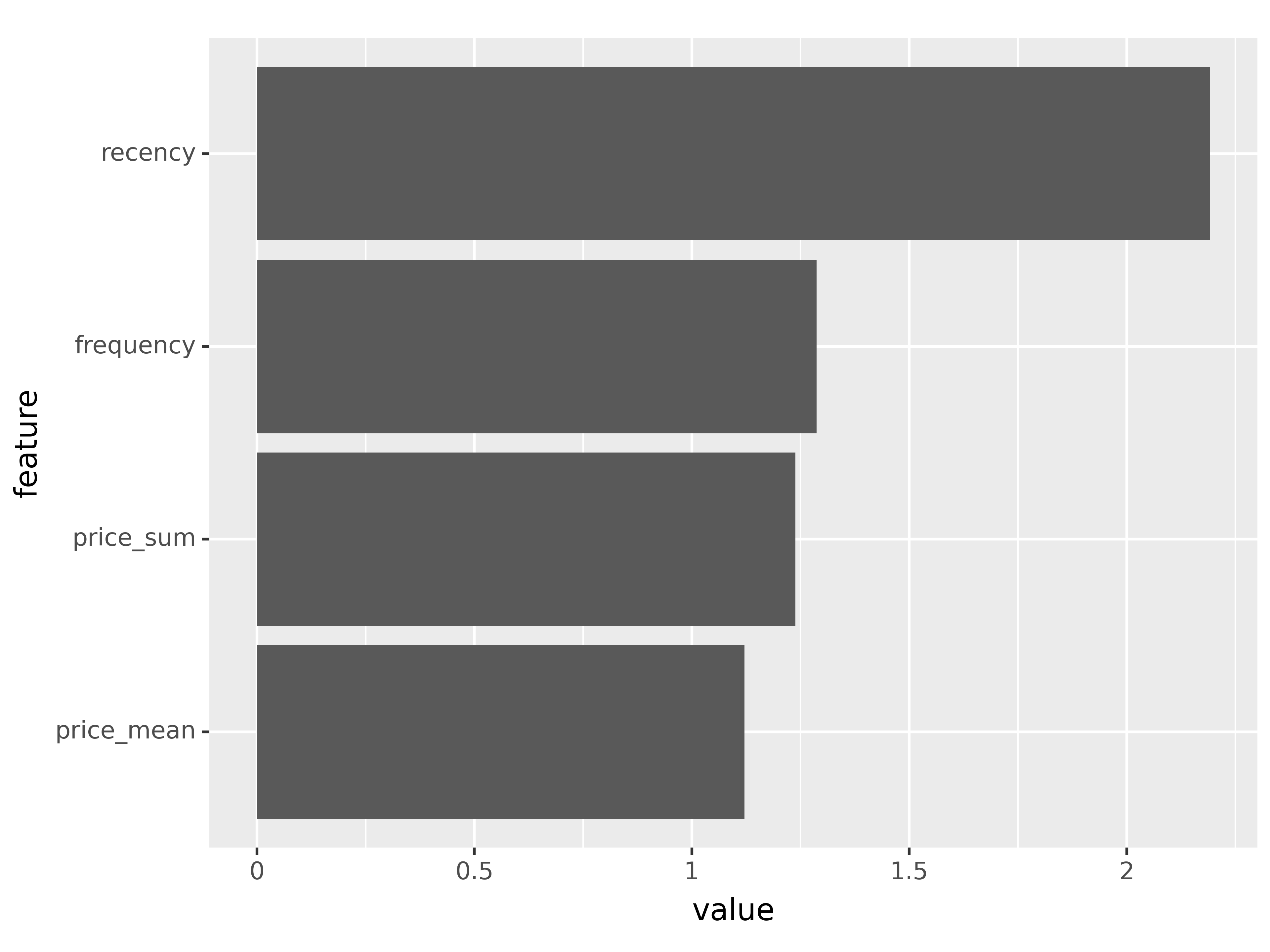 

<Figure Size: (1920 x 1440)>

In terms of the probability of future spend, if a customer has spent recently and frequently, then these are strong indicators. The amount spent and average spend are not considered to be important by the model.

7. Pickle (save) our predictions, features, and models

# Combine our predictions
predictions_df = pd.concat(
    [
        pd.DataFrame(predictions_reg).set_axis(['pred_spend'], axis=1),
        pd.DataFrame(predictions_clf)[[1]].set_axis(['pred_prob'], axis=1),
        features_df.reset_index()
    ], 
    axis=1
)
predictions_df

	pred_spend	pred_prob	fullVisitorId	recency	frequency	price_sum	price_mean	spend_90_total	spend_90_flag
0	1.186358	0.024005	0000213131142648941	-5.0	1	33.59	33.590000	0.0	0.0
1	0.264711	0.000514	0002871498069867123	-253.0	1	5.99	5.990000	0.0	0.0
2	0.264711	0.000490	0003450834640354121	-197.0	5	57.95	11.590000	0.0	0.0
3	0.264711	0.000253	000435324061339869	-195.0	1	44.79	44.790000	0.0	0.0
4	0.264711	0.000409	0007617910709180468	-142.0	1	18.99	18.990000	0.0	0.0
...	...	...	...	...	...	...	...	...	...
7473	0.361555	0.012704	9991633376050115277	-75.0	1	33.59	33.590000	0.0	0.0
7474	0.264711	0.000526	9994767073213036303	-267.0	6	51.94	8.656667	0.0	0.0
7475	0.264711	0.000852	9997409246962677759	-146.0	5	32.36	6.472000	0.0	0.0
7476	0.264711	0.000980	9998597322098588317	-275.0	2	3.24	1.620000	0.0	0.0
7477	0.264711	0.000581	9998996003043230595	-168.0	2	59.98	29.990000	0.0	0.0

7478 rows × 9 columns

import pickle

with open("artifacts/predictions_df.pkl", "wb") as file:
    pickle.dump(predictions_df, file, protocol=4)

# Pickle our predictions
predictions_df.to_pickle("artifacts/predictions_df.pkl")

with open("artifacts/imp_spend_amount_df.pkl", "wb") as file:
    pickle.dump(imp_spend_amount_df, file, protocol=4)

with open("artifacts/imp_spend_prob_df.pkl", "wb") as file:
    pickle.dump(imp_spend_prob_df, file, protocol=4)

### Save our Feature Importances
imp_spend_amount_df.to_pickle("artifacts/imp_spend_amount_df.pkl")
imp_spend_prob_df.to_pickle("artifacts/imp_spend_prob_df.pkl")

### Save Models
joblib.dump(xgb_reg_model, 'artifacts/xgb_reg_model.pkl')
joblib.dump(xgb_clf_model, 'artifacts/xgb_clf_model.pkl')

model = joblib.load('artifacts/xgb_reg_model.pkl')
model.predict(X)

array([1.1863576 , 0.26471087, 0.26471087, ..., 0.26471087, 0.26471087,
       0.26471087], dtype=float32)

8. Actionable outcomes

8.1 Which customers have the highest spend probability in next 90-days?

• Target for new products similar to what they have purchased in the past.

predictions_df \
    .sort_values('pred_prob', ascending=False)

	pred_spend	pred_prob	fullVisitorId	recency	frequency	price_sum	price_mean	spend_90_total	spend_90_flag
3747	103.428444	0.849751	4984366501121503466	-23.0	55	320.57	5.828545	258.50	1.0
6156	258.405396	0.836090	8197879643797712877	-7.0	65	2052.37	31.574923	657.03	1.0
1430	225.969971	0.827522	1957458976293878100	-14.0	109	2333.35	21.406881	338.26	1.0
3724	34.220909	0.806135	4950411203281265700	0.0	23	120.62	5.244348	92.35	1.0
5888	69.604485	0.782023	7813149961404844386	0.0	48	1906.50	39.718750	175.79	1.0
...	...	...	...	...	...	...	...	...	...
1307	0.264711	0.000214	1799218307967476916	-202.0	1	16.99	16.990000	0.00	0.0
2573	0.264711	0.000214	3461504855909388246	-206.0	1	16.99	16.990000	0.00	0.0
4435	0.264711	0.000214	5844997119511169482	-216.0	1	18.99	18.990000	0.00	0.0
6228	0.264711	0.000214	8292732469404938023	-227.0	1	16.99	16.990000	0.00	0.0
3206	0.264711	0.000214	4259785355346404932	-210.0	1	18.99	18.990000	0.00	0.0

7478 rows × 9 columns

We can see that the model seems to be working well in terms of identifying those customers that are likely to spend in the next-90 days. The top 5 customers above ranked by probability of spend all actually spent. Conversely, the bottom 5 customers didn’t spend.

8.2 Which customers have recently purchased (within 90 days) but are unlikely to buy (probability less than 30%)?

• Incentivize actions to increase probability.
• Provide discounts, encourage referring a friend, nurture by letting them know what’s coming.

predictions_df \
    [
        predictions_df['recency'] > -90
    ] \
    [
        predictions_df['pred_prob'] < 0.30
    ] \
    .sort_values('pred_prob', ascending=False)

	pred_spend	pred_prob	fullVisitorId	recency	frequency	price_sum	price_mean	spend_90_total	spend_90_flag
2384	2.970100	0.299618	3197533100947860058	-33.0	7	153.44	21.920	86.54	1.0
419	4.334545	0.291470	0554420125524525961	-10.0	3	52.77	17.590	172.37	1.0
3406	2.242671	0.291250	4515197722749947898	-3.0	2	28.78	14.390	0.00	0.0
1861	2.242671	0.291250	2518379317255532090	-3.0	2	28.78	14.390	28.78	1.0
5688	3.153815	0.290945	7548511681521037018	-2.0	4	33.98	8.495	42.97	1.0
...	...	...	...	...	...	...	...	...	...
6446	0.594005	0.001943	8590369633898567459	-35.0	1	2.39	2.390	0.00	0.0
5561	0.594005	0.001943	7390358029425621068	-35.0	1	1.99	1.990	0.00	0.0
2165	0.361555	0.001671	293387037477216156	-72.0	1	1.99	1.990	0.00	0.0
2666	0.361555	0.001671	3573113591289892546	-74.0	1	1.99	1.990	0.00	0.0
1490	0.361555	0.001671	2037170738057013329	-73.0	1	1.99	1.990	0.00	0.0

2324 rows × 9 columns

8.3 Missed opportunities: Big spenders that could be unlocked

• Send bundle offers encouraging volume purchases
• Focus on missed opportunities

# identify those customers predicted to spend but did not
predictions_df \
    [
        predictions_df['spend_90_total'] == 0.0
    ] \
    .sort_values('pred_spend', ascending=False) 

	pred_spend	pred_prob	fullVisitorId	recency	frequency	price_sum	price_mean	spend_90_total	spend_90_flag
2955	81.598740	0.126212	3955127543379144640	-2.0	8	358.32	44.790000	0.0	0.0
2565	33.736187	0.063039	3449924104971285851	-91.0	14	483.86	34.561429	0.0	0.0
5696	33.736187	0.085885	7561014297963838461	-58.0	18	522.82	29.045556	0.0	0.0
2927	30.029305	0.017011	3916992730920009646	-64.0	7	416.73	59.532857	0.0	0.0
4026	30.029305	0.009925	5349155616428631188	-76.0	13	391.87	30.143846	0.0	0.0
...	...	...	...	...	...	...	...	...	...
1767	-0.646184	0.025690	2396848817613598114	-59.0	44	1416.56	32.194545	0.0	0.0
5808	-0.646184	0.023305	7713012430069756739	-62.0	18	783.82	43.545556	0.0	0.0
751	-0.646184	0.017749	1045033759778661078	-86.0	22	657.38	29.880909	0.0	0.0
7001	-0.646184	0.013225	9349161317881541522	-50.0	29	896.71	30.921034	0.0	0.0
3873	-0.925417	0.007162	5149788969578895545	-66.0	9	340.71	37.856667	0.0	0.0

7356 rows × 9 columns

9. Communication of findings

9.1 e-commerce analytics dashboard using Dash for viewing locally

We can create an interactive analytics dashboard which can be shared with the Marketing Department to enable targeted campaigns to be launched, by following these 3 steps:

1. Create a virtual environment from the command line :

    conda env create -f environment.yml

This minimizes the risk of conflicting package dependencies or dependency hell! If you do end up down there then you can refer to the documentation. Good luck!

2. Activate the environment:

    conda activate google_merch_clv (this is the name specified in the yaml file below - can change this as desired)

3. Launch the app:

    python app.py    

The dashboard can then be viewed by visiting http://127.0.0.1:8050/ in your web browser.

9.2 Deployment of Dash e-commerce app

Now that we have tested our app and it runs successfully locally, it’s time to deploy it! There are a variety of platforms around, most have some kind of pay wall. Python Anywhere offer a basic free hosting service but tou might find you need a bit more resource. At the time of writing $7/$8 per month allows you to have two apps hosted and gives you 2000s of CPU usage and 2.0GB of file storage.

It has a very user-friendly interface and after reviewing some online video tutorials and debugging using the support forums and stackoverflow, i was able to get my app running.

10. Key takeaways

This project demonstrated my proficiency in:

• business analytics: the project was framed by two business problems/questions which are relevant to ecommerce businesses
• SQL: transform a complex real-life BigData datset with nested fields, into meaningful insights with regard to customer behaviour
• pandas: data cleansing and wrangling
• machine learning: created a BASELINE regression and classification model and performed feature engineering to enhance model performance
• visualization: using the plotly and plotnine libraries
• app creation : deployment of an interactive Dash app

At the time of writing I am currently working on a customer segmentation and recommendation engine project which makes use of the same dataset.