Data Engineering Zoomcamp - Final Project

DE Zoomcamp - Final Project

Spotify 1.2 million - Project Overview

It’s time to pull everything together I’ve learned during this course and complete an end to end data pipeline project. As a musician I decided to chose a dataset of personal interest to me :

• audio features of over 1.2 million songs obtained with the Spotify API

Acknowledgements to Rodolfo Figueroa for curating the dataset. Kaggle assigned the dataset a solid Usability score of 8.24 which is a good starting point. Whilst this is primarily a data engineering project I will also be carrying out some data pre-processing.

Data logistics is no different from any other form of logistics, in that it will not be possible to move our data from source, in my case a raw csv file held on Kaggle to destination, in my case Looker Studio without a few bumps along the way. But by carrying out some preliminary data exploration, and harnessing workflow orchestration tools, we can make the journey as smooth as possible.

So sit back and enjoy the ride ;)

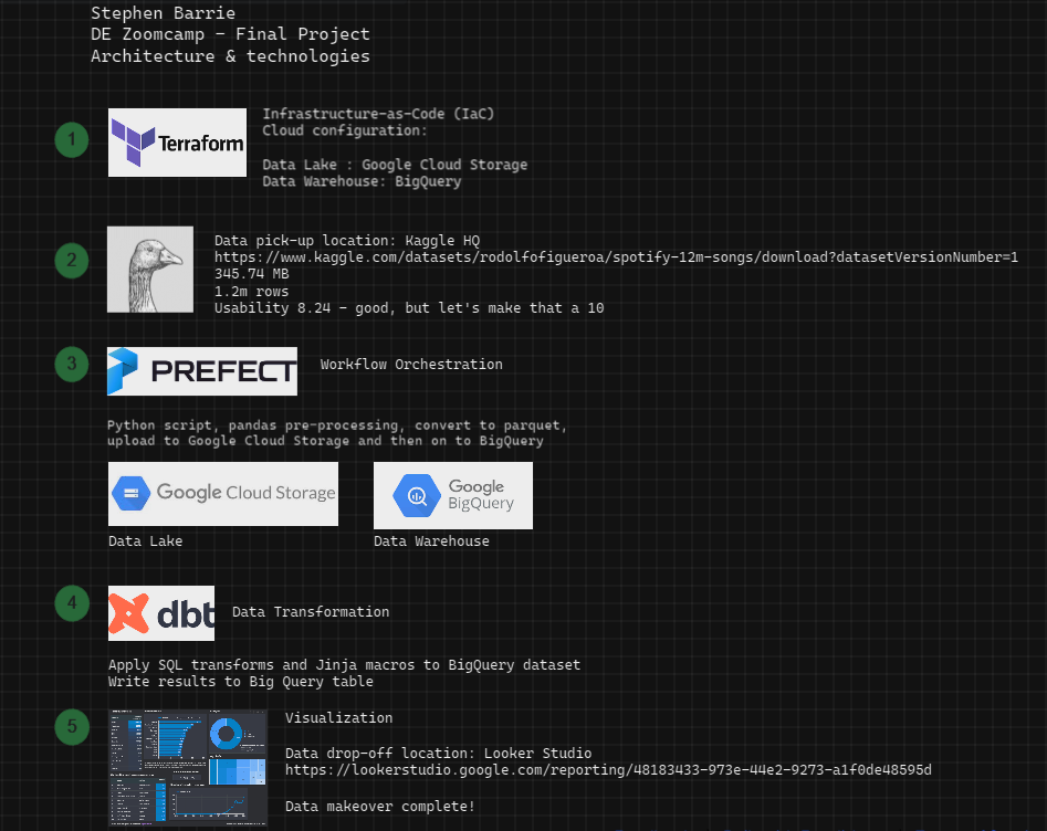
0. Project architecture & technologies

Outlined below is an overview of the architecture and technologies that I will be using to unveil some insights from the raw data.

Architecture_Technologies.png

1. Set up & configuration

Reproducability

I use Unbuntu on Windows 20.04.5 and like to run things locally from the command line wherever possible, however this project does make use of cloud applications.

A pre-requisite for reproducability of this project is having a Google Cloud account. I set mine up at the beginning of this course. You can follow these instructions to get up and running.

For the purposes of this specific project, I used Terraform (Infrastructure-as-Code) to automate my cloud resources configuration. I had already set this up locally at the beginning of the course and so only required the following two files to configure my data bucket in Google Cloud Storage, and my Data Warehouse, BigQuery.

main.tf

terraform {
  required_version = ">= 1.0"
  backend "local" {}  # Can change from "local" to "gcs" (for google) or "s3" (for aws), if you would like to preserve your tf-state online
  required_providers {
    google = {
      source  = "hashicorp/google"
    }
  }
}

provider "google" {
  project = var.project
  region = var.region
  // credentials = file(var.credentials)  # Use this if you do not want to set env-var GOOGLE_APPLICATION_CREDENTIALS
}

# Data Lake Bucket
# Ref: https://registry.terraform.io/providers/hashicorp/google/latest/docs/resources/storage_bucket
resource "google_storage_bucket" "data-lake-bucket" {
  name          = "${local.data_lake_bucket}_${var.project}" # Concatenating DL bucket & Project name for unique naming
  location      = var.region

  # Optional, but recommended settings:
  storage_class = var.storage_class
  uniform_bucket_level_access = true

  versioning {
    enabled     = true
  }

  lifecycle_rule {
    action {
      type = "Delete"
    }
    condition {
      age = 30  // days
    }
  }

  force_destroy = true
}

# DWH
# Ref: https://registry.terraform.io/providers/hashicorp/google/latest/docs/resources/bigquery_dataset
resource "google_bigquery_dataset" "dataset" {
  dataset_id = var.BQ_DATASET
  project    = var.project
  location   = var.region
}

variables.tf

locals {
  data_lake_bucket = "spotify"
}

variable "project" {
  description = "de-zoomcamp-project137"
}

variable "region" {
  description = "Region for GCP resources. Choose as per your location: https://cloud.google.com/about/locations"
  default = "europe-west6"
  type = string
}

variable "storage_class" {
  description = "Storage class type for your bucket. Check official docs for more info."
  default = "STANDARD"
}

variable "BQ_DATASET" {
  description = "BigQuery Dataset that raw data (from GCS) will be written to"
  type = string
  default = "spotify"
}

Once you have configured these files you can simply run the following prompts from the command line :

Refresh service-account’s auth-token for this session :

gcloud auth application-default login

Initialize state file :

terraform init

Check changes to new infra plan :

terraform plan -var="project=<your-gcp-project-id>"

Asks for approval to the proposed plan, and applies changes to cloud :

terraform apply

For further assistance refer to this detailed guide on Local Setup for Terraform and GCP.

2. Data-pick up & preproceesing

I was unable to download the file using the link address to the file on Kaggle :

kaggle_download.PNG

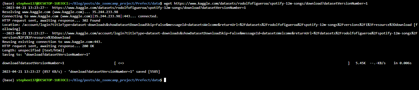
As a workaround I resorted to clicking on the Download icon to save the file locally. We can access the file size (memory) and number of rows from the command line using the following commands :

du -h <file_name>
wc -l <file_name>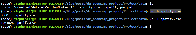  

spotify_csv.PNG

Let’s get to know our data :

import pandas as pd
df = pd.read_csv('Prefect/data/spotify.csv')
df.head()

	id	name	album	album_id	artists	artist_ids	track_number	disc_number	explicit	danceability	...	speechiness	acousticness	instrumentalness	liveness	valence	tempo	duration_ms	time_signature	year	release_date
0	7lmeHLHBe4nmXzuXc0HDjk	Testify	The Battle Of Los Angeles	2eia0myWFgoHuttJytCxgX	['Rage Against The Machine']	['2d0hyoQ5ynDBnkvAbJKORj']	1	1	False	0.470	...	0.0727	0.02610	0.000011	0.3560	0.503	117.906	210133	4.0	1999	1999-11-02
1	1wsRitfRRtWyEapl0q22o8	Guerrilla Radio	The Battle Of Los Angeles	2eia0myWFgoHuttJytCxgX	['Rage Against The Machine']	['2d0hyoQ5ynDBnkvAbJKORj']	2	1	True	0.599	...	0.1880	0.01290	0.000071	0.1550	0.489	103.680	206200	4.0	1999	1999-11-02
2	1hR0fIFK2qRG3f3RF70pb7	Calm Like a Bomb	The Battle Of Los Angeles	2eia0myWFgoHuttJytCxgX	['Rage Against The Machine']	['2d0hyoQ5ynDBnkvAbJKORj']	3	1	False	0.315	...	0.4830	0.02340	0.000002	0.1220	0.370	149.749	298893	4.0	1999	1999-11-02
3	2lbASgTSoDO7MTuLAXlTW0	Mic Check	The Battle Of Los Angeles	2eia0myWFgoHuttJytCxgX	['Rage Against The Machine']	['2d0hyoQ5ynDBnkvAbJKORj']	4	1	True	0.440	...	0.2370	0.16300	0.000004	0.1210	0.574	96.752	213640	4.0	1999	1999-11-02
4	1MQTmpYOZ6fcMQc56Hdo7T	Sleep Now In the Fire	The Battle Of Los Angeles	2eia0myWFgoHuttJytCxgX	['Rage Against The Machine']	['2d0hyoQ5ynDBnkvAbJKORj']	5	1	False	0.426	...	0.0701	0.00162	0.105000	0.0789	0.539	127.059	205600	4.0	1999	1999-11-02

5 rows × 24 columns

On first look the dataset appears to be fairly clean - the artists name are wrapped in [' '] and some of the values for track features are taken to a large number of decimal places. We’ll include these clean up as a flow as part of a data ingestion script using Prefect which will read the csv, convert to parquet format, and upload to Google Cloud Storage.

df.info()

<class 'pandas.core.frame.DataFrame'>
RangeIndex: 1204025 entries, 0 to 1204024
Data columns (total 24 columns):
 #   Column            Non-Null Count    Dtype  
---  ------            --------------    -----  
 0   id                1204025 non-null  object 
 1   name              1204025 non-null  object 
 2   album             1204025 non-null  object 
 3   album_id          1204025 non-null  object 
 4   artists           1204025 non-null  object 
 5   artist_ids        1204025 non-null  object 
 6   track_number      1204025 non-null  int64  
 7   disc_number       1204025 non-null  int64  
 8   explicit          1204025 non-null  bool   
 9   danceability      1204025 non-null  float64
 10  energy            1204025 non-null  float64
 11  key               1204025 non-null  int64  
 12  loudness          1204025 non-null  float64
 13  mode              1204025 non-null  int64  
 14  speechiness       1204025 non-null  float64
 15  acousticness      1204025 non-null  float64
 16  instrumentalness  1204025 non-null  float64
 17  liveness          1204025 non-null  float64
 18  valence           1204025 non-null  float64
 19  tempo             1204025 non-null  float64
 20  duration_ms       1204025 non-null  int64  
 21  time_signature    1204025 non-null  float64
 22  year              1204025 non-null  int64  
 23  release_date      1204025 non-null  object 
dtypes: bool(1), float64(10), int64(6), object(7)
memory usage: 212.4+ MB

df.info gives us the number of entries, in our case 1,204,025, columns 24, number of non-null entries for each column (in our case same as number of entries, so no NULL values), and the datatype for each column.

It is vital to ensure that the data is in the correct format for our analytics project. Off the bat, I can see that the year and release_date datatypes will need to be converted to a date type.

df.describe()

	track_number	disc_number	danceability	energy	key	loudness	mode	speechiness	acousticness	instrumentalness	liveness	valence	tempo	duration_ms	time_signature	year
count	1.204025e+06	1.204025e+06	1.204025e+06	1.204025e+06	1.204025e+06	1.204025e+06	1.204025e+06	1.204025e+06	1.204025e+06	1.204025e+06	1.204025e+06	1.204025e+06	1.204025e+06	1.204025e+06	1.204025e+06	1.204025e+06
mean	7.656352e+00	1.055906e+00	4.930565e-01	5.095363e-01	5.194151e+00	-1.180870e+01	6.714595e-01	8.438219e-02	4.467511e-01	2.828605e-01	2.015994e-01	4.279866e-01	1.176344e+02	2.488399e+05	3.832494e+00	2.007328e+03
std	5.994977e+00	2.953752e-01	1.896694e-01	2.946839e-01	3.536731e+00	6.982132e+00	4.696827e-01	1.159914e-01	3.852014e-01	3.762844e-01	1.804591e-01	2.704846e-01	3.093705e+01	1.622104e+05	5.611826e-01	1.210117e+01
min	1.000000e+00	1.000000e+00	0.000000e+00	0.000000e+00	0.000000e+00	-6.000000e+01	0.000000e+00	0.000000e+00	0.000000e+00	0.000000e+00	0.000000e+00	0.000000e+00	0.000000e+00	1.000000e+03	0.000000e+00	0.000000e+00
25%	3.000000e+00	1.000000e+00	3.560000e-01	2.520000e-01	2.000000e+00	-1.525400e+01	0.000000e+00	3.510000e-02	3.760000e-02	7.600000e-06	9.680000e-02	1.910000e-01	9.405400e+01	1.740900e+05	4.000000e+00	2.002000e+03
50%	7.000000e+00	1.000000e+00	5.010000e-01	5.240000e-01	5.000000e+00	-9.791000e+00	1.000000e+00	4.460000e-02	3.890000e-01	8.080000e-03	1.250000e-01	4.030000e-01	1.167260e+02	2.243390e+05	4.000000e+00	2.009000e+03
75%	1.000000e+01	1.000000e+00	6.330000e-01	7.660000e-01	8.000000e+00	-6.717000e+00	1.000000e+00	7.230000e-02	8.610000e-01	7.190000e-01	2.450000e-01	6.440000e-01	1.370460e+02	2.858400e+05	4.000000e+00	2.015000e+03
max	5.000000e+01	1.300000e+01	1.000000e+00	1.000000e+00	1.100000e+01	7.234000e+00	1.000000e+00	9.690000e-01	9.960000e-01	1.000000e+00	1.000000e+00	1.000000e+00	2.489340e+02	6.061090e+06	5.000000e+00	2.020000e+03

This gives us a very useful overview of our dataset and can highlight anomalies worthy of further investigation. min and max in particular allow us to make a very quick sense check of the range of the data, and might unveil potential outliers.

Take a look at our year column - the range of values are 0 to 2020. So, it looks like imputed values have been used where information was not available. This may cause problems later when we attempt to convert the datatype for year which is currently int64.

We can use .iloc to access a group of rows and columns by index or .loc to access a group of rows and columns by name :

df.loc[df['year'] == 0 ]

	id	name	album	album_id	artists	artist_ids	track_number	disc_number	explicit	danceability	...	speechiness	acousticness	instrumentalness	liveness	valence	tempo	duration_ms	time_signature	year	release_date
815351	035h5flqzwF6I5CTfsdHPA	Jimmy Neutron	Optimism 2	211vSdhxt58A943r9QWRKo	['iCizzle']	['7arv4matK2uKJrdtPSxU4i']	1	1	False	0.795	...	0.0519	0.01560	0.439	0.0860	0.389	109.985	183000	4.0	0	0000
815352	49x05fLGDKCsCUA7CG0VpY	I Luv You	Optimism 2	211vSdhxt58A943r9QWRKo	['iCizzle']	['7arv4matK2uKJrdtPSxU4i']	2	1	False	0.762	...	0.0950	0.88700	0.909	0.1060	0.728	92.962	145161	4.0	0	0000
815353	4mNLlSoZOqoPauBAF3bIpx	My Heart	Optimism 2	211vSdhxt58A943r9QWRKo	['iCizzle']	['7arv4matK2uKJrdtPSxU4i']	3	1	False	0.671	...	0.0662	0.00956	0.902	0.0455	0.893	97.865	176561	4.0	0	0000
815354	7w5iwI0wnIiopbCFNe1Txo	I Am (Invincible)	Optimism 2	211vSdhxt58A943r9QWRKo	['iCizzle']	['7arv4matK2uKJrdtPSxU4i']	4	1	False	0.759	...	0.1280	0.00544	0.895	0.0538	0.537	89.989	192000	4.0	0	0000
815355	2Tfy2R2uiWVwxHQUT6oGNp	Flower Power	Optimism 2	211vSdhxt58A943r9QWRKo	['iCizzle']	['7arv4matK2uKJrdtPSxU4i']	5	1	False	0.657	...	0.2810	0.01800	0.245	0.2410	0.964	179.904	138666	4.0	0	0000
815356	05cTbSPQyha6z7opYwH67O	Heard It Low	Optimism 2	211vSdhxt58A943r9QWRKo	['iCizzle']	['7arv4matK2uKJrdtPSxU4i']	6	1	False	0.728	...	0.0673	0.00785	0.275	0.0865	0.662	90.010	138667	4.0	0	0000
815357	1fYK5xB8csOXVEqApkzzm0	Hangin On	Optimism 2	211vSdhxt58A943r9QWRKo	['iCizzle']	['7arv4matK2uKJrdtPSxU4i']	7	1	False	0.822	...	0.0758	0.11500	0.881	0.1210	0.766	119.998	142620	4.0	0	0000
815358	4G51c7cWzB6CLaRq9sYj2w	God Loves You	Optimism 2	211vSdhxt58A943r9QWRKo	['iCizzle']	['7arv4matK2uKJrdtPSxU4i']	8	1	False	0.845	...	0.0662	0.00274	0.548	0.0393	0.472	120.090	161000	4.0	0	0000
815359	45fcUAjXlzDxTwSzoUaO6l	You In My Life	Optimism 2	211vSdhxt58A943r9QWRKo	['iCizzle']	['7arv4matK2uKJrdtPSxU4i']	9	1	False	0.957	...	0.0623	0.13300	0.857	0.0968	0.258	112.987	214867	4.0	0	0000
815360	35TcKSN5hsGcZLrFPkUvIv	I Wonder	Optimism 2	211vSdhxt58A943r9QWRKo	['iCizzle']	['7arv4matK2uKJrdtPSxU4i']	10	1	False	0.659	...	0.0581	0.00196	0.854	0.3710	0.877	146.020	180822	4.0	0	0000

10 rows × 24 columns

So, the tracks from the album Optimism 2 by the artist iCizzle have been given a year value of 0. A quick internet search and we can see the year should be 2018. Now that we have located our anomalies, we can update these values using .loc :

df.loc[815351:815360,'year'] = 2018

Let’s check that worked :

df.loc[815351:815360] 

	id	name	album	album_id	artists	artist_ids	track_number	disc_number	explicit	danceability	...	speechiness	acousticness	instrumentalness	liveness	valence	tempo	duration_ms	time_signature	year	release_date
815351	035h5flqzwF6I5CTfsdHPA	Jimmy Neutron	Optimism 2	211vSdhxt58A943r9QWRKo	['iCizzle']	['7arv4matK2uKJrdtPSxU4i']	1	1	False	0.795	...	0.0519	0.01560	0.439	0.0860	0.389	109.985	183000	4.0	2018	0000
815352	49x05fLGDKCsCUA7CG0VpY	I Luv You	Optimism 2	211vSdhxt58A943r9QWRKo	['iCizzle']	['7arv4matK2uKJrdtPSxU4i']	2	1	False	0.762	...	0.0950	0.88700	0.909	0.1060	0.728	92.962	145161	4.0	2018	0000
815353	4mNLlSoZOqoPauBAF3bIpx	My Heart	Optimism 2	211vSdhxt58A943r9QWRKo	['iCizzle']	['7arv4matK2uKJrdtPSxU4i']	3	1	False	0.671	...	0.0662	0.00956	0.902	0.0455	0.893	97.865	176561	4.0	2018	0000
815354	7w5iwI0wnIiopbCFNe1Txo	I Am (Invincible)	Optimism 2	211vSdhxt58A943r9QWRKo	['iCizzle']	['7arv4matK2uKJrdtPSxU4i']	4	1	False	0.759	...	0.1280	0.00544	0.895	0.0538	0.537	89.989	192000	4.0	2018	0000
815355	2Tfy2R2uiWVwxHQUT6oGNp	Flower Power	Optimism 2	211vSdhxt58A943r9QWRKo	['iCizzle']	['7arv4matK2uKJrdtPSxU4i']	5	1	False	0.657	...	0.2810	0.01800	0.245	0.2410	0.964	179.904	138666	4.0	2018	0000
815356	05cTbSPQyha6z7opYwH67O	Heard It Low	Optimism 2	211vSdhxt58A943r9QWRKo	['iCizzle']	['7arv4matK2uKJrdtPSxU4i']	6	1	False	0.728	...	0.0673	0.00785	0.275	0.0865	0.662	90.010	138667	4.0	2018	0000
815357	1fYK5xB8csOXVEqApkzzm0	Hangin On	Optimism 2	211vSdhxt58A943r9QWRKo	['iCizzle']	['7arv4matK2uKJrdtPSxU4i']	7	1	False	0.822	...	0.0758	0.11500	0.881	0.1210	0.766	119.998	142620	4.0	2018	0000
815358	4G51c7cWzB6CLaRq9sYj2w	God Loves You	Optimism 2	211vSdhxt58A943r9QWRKo	['iCizzle']	['7arv4matK2uKJrdtPSxU4i']	8	1	False	0.845	...	0.0662	0.00274	0.548	0.0393	0.472	120.090	161000	4.0	2018	0000
815359	45fcUAjXlzDxTwSzoUaO6l	You In My Life	Optimism 2	211vSdhxt58A943r9QWRKo	['iCizzle']	['7arv4matK2uKJrdtPSxU4i']	9	1	False	0.957	...	0.0623	0.13300	0.857	0.0968	0.258	112.987	214867	4.0	2018	0000
815360	35TcKSN5hsGcZLrFPkUvIv	I Wonder	Optimism 2	211vSdhxt58A943r9QWRKo	['iCizzle']	['7arv4matK2uKJrdtPSxU4i']	10	1	False	0.659	...	0.0581	0.00196	0.854	0.3710	0.877	146.020	180822	4.0	2018	0000

10 rows × 24 columns

We have successfully updated the release year to 2018. Let’s check the range of dates once more :

df.year.describe()

count    1.204025e+06
mean     2.007345e+03
std      1.062889e+01
min      1.900000e+03
25%      2.002000e+03
50%      2.009000e+03
75%      2.015000e+03
max      2.020000e+03
Name: year, dtype: float64

So, the minimum year is now 1900. Again, this seems like it might be another imputed value. Let’s check :

df.loc[df['year'] == 1900 ]

	id	name	album	album_id	artists	artist_ids	track_number	disc_number	explicit	danceability	...	speechiness	acousticness	instrumentalness	liveness	valence	tempo	duration_ms	time_signature	year	release_date
450071	3xPatAieFSuGIuQfHMDvSw	Arabian Waltz	Arabian Waltz	1ggHQJ48NFfYhGu6VznK8K	['Rabih Abou-Khalil']	['7cM9Y2LNnnmmqivaEuH8vT']	1	1	False	0.533	...	0.0576	0.875	0.859	0.0887	0.8350	115.746	493867	3.0	1900	1900-01-01
450072	5vpx0WtYVtKOFu4V65NkUi	Dreams Of A Dying City	Arabian Waltz	1ggHQJ48NFfYhGu6VznK8K	['Rabih Abou-Khalil']	['7cM9Y2LNnnmmqivaEuH8vT']	2	1	False	0.476	...	0.0334	0.843	0.893	0.1060	0.5710	92.340	730667	1.0	1900	1900-01-01
450073	0G7vBbeWCcRISsHwcivFgl	Ornette Never Sleeps	Arabian Waltz	1ggHQJ48NFfYhGu6VznK8K	['Rabih Abou-Khalil']	['7cM9Y2LNnnmmqivaEuH8vT']	3	1	False	0.605	...	0.0457	0.912	0.693	0.1170	0.7250	139.820	421760	4.0	1900	1900-01-01
450074	6YjrfDT2TPp6pflsCSBHPH	Georgina	Arabian Waltz	1ggHQJ48NFfYhGu6VznK8K	['Rabih Abou-Khalil']	['7cM9Y2LNnnmmqivaEuH8vT']	4	1	False	0.406	...	0.0433	0.849	0.866	0.1020	0.6200	93.729	672707	4.0	1900	1900-01-01
450075	2Nq317w5G1gmuhilTCiiqR	No Visa	Arabian Waltz	1ggHQJ48NFfYhGu6VznK8K	['Rabih Abou-Khalil']	['7cM9Y2LNnnmmqivaEuH8vT']	5	1	False	0.577	...	0.0430	0.936	0.865	0.0999	0.5010	96.415	601027	4.0	1900	1900-01-01
450076	6PzeE7vvynVguz04STK6RL	The Pain After	Arabian Waltz	1ggHQJ48NFfYhGu6VznK8K	['Rabih Abou-Khalil']	['7cM9Y2LNnnmmqivaEuH8vT']	6	1	False	0.291	...	0.0477	0.956	0.939	0.1460	0.0959	71.087	566840	3.0	1900	1900-01-01
459980	4DZ63H1bRMmiTcXiQhERxv	Catania	Al-Jadida	2T6FKoeG7EXR0WAsFyXbSq	['Rabih Abou-Khalil']	['7cM9Y2LNnnmmqivaEuH8vT']	1	1	False	0.465	...	0.0742	0.414	0.089	0.0936	0.3790	163.939	465000	5.0	1900	1900-01-01
459981	6QqZn286ICbbhTjNBPlgNY	Nashwa	Al-Jadida	2T6FKoeG7EXR0WAsFyXbSq	['Rabih Abou-Khalil']	['7cM9Y2LNnnmmqivaEuH8vT']	2	1	False	0.436	...	0.0683	0.802	0.758	0.1070	0.1580	171.006	578000	5.0	1900	1900-01-01
459982	5Mw5YkQkHuGqYQL5XMrUOI	An Evening With Jerry	Al-Jadida	2T6FKoeG7EXR0WAsFyXbSq	['Rabih Abou-Khalil']	['7cM9Y2LNnnmmqivaEuH8vT']	3	1	False	0.511	...	0.0350	0.211	0.550	0.1900	0.2530	144.884	423000	4.0	1900	1900-01-01
459983	4SNCi2xa3dkM0HPTQ1AFBP	When The Lights Go Out	Al-Jadida	2T6FKoeG7EXR0WAsFyXbSq	['Rabih Abou-Khalil']	['7cM9Y2LNnnmmqivaEuH8vT']	4	1	False	0.414	...	0.0602	0.826	0.880	0.1180	0.0783	154.842	433960	4.0	1900	1900-01-01
459984	1XEbjKZygiDllK5WpEB73O	Story Teller	Al-Jadida	2T6FKoeG7EXR0WAsFyXbSq	['Rabih Abou-Khalil']	['7cM9Y2LNnnmmqivaEuH8vT']	5	1	False	0.595	...	0.0458	0.537	0.658	0.3540	0.3370	109.885	532173	4.0	1900	1900-01-01
459985	5V4pmHLdq0fhEw5DjkaW2w	Ornette Never Sleps	Al-Jadida	2T6FKoeG7EXR0WAsFyXbSq	['Rabih Abou-Khalil']	['7cM9Y2LNnnmmqivaEuH8vT']	6	1	False	0.470	...	0.0569	0.593	0.914	0.1050	0.8140	158.412	243867	3.0	1900	1900-01-01
459986	6BeB08lGiB6zd8Fn7BBhb1	Nadim	Al-Jadida	2T6FKoeG7EXR0WAsFyXbSq	['Rabih Abou-Khalil']	['7cM9Y2LNnnmmqivaEuH8vT']	7	1	False	0.474	...	0.0532	0.401	0.561	0.0785	0.3010	162.807	513000	4.0	1900	1900-01-01
459987	1WRapjF1HuE2rXUVBGKXXt	Wishing Well	Al-Jadida	2T6FKoeG7EXR0WAsFyXbSq	['Rabih Abou-Khalil']	['7cM9Y2LNnnmmqivaEuH8vT']	8	1	False	0.521	...	0.0594	0.828	0.792	0.1040	0.2420	127.288	325000	4.0	1900	1900-01-01

14 rows × 24 columns

So, the tracks with a year value of 1900 all relate to the artist Rabih Abou-Khalil. Another quick internet search and we can see the actual year for the album Al-Jadida is 1991 and for the album Arabian Waltz is 1996.

Let’s update these :

df.loc[450071:450076,'year'] = 1996
df.loc[459980:459987,'year'] = 1991

and check that’s worked :

df.loc[450071:450076]

	id	name	album	album_id	artists	artist_ids	track_number	disc_number	explicit	danceability	...	speechiness	acousticness	instrumentalness	liveness	valence	tempo	duration_ms	time_signature	year	release_date
450071	3xPatAieFSuGIuQfHMDvSw	Arabian Waltz	Arabian Waltz	1ggHQJ48NFfYhGu6VznK8K	['Rabih Abou-Khalil']	['7cM9Y2LNnnmmqivaEuH8vT']	1	1	False	0.533	...	0.0576	0.875	0.859	0.0887	0.8350	115.746	493867	3.0	1996	1900-01-01
450072	5vpx0WtYVtKOFu4V65NkUi	Dreams Of A Dying City	Arabian Waltz	1ggHQJ48NFfYhGu6VznK8K	['Rabih Abou-Khalil']	['7cM9Y2LNnnmmqivaEuH8vT']	2	1	False	0.476	...	0.0334	0.843	0.893	0.1060	0.5710	92.340	730667	1.0	1996	1900-01-01
450073	0G7vBbeWCcRISsHwcivFgl	Ornette Never Sleeps	Arabian Waltz	1ggHQJ48NFfYhGu6VznK8K	['Rabih Abou-Khalil']	['7cM9Y2LNnnmmqivaEuH8vT']	3	1	False	0.605	...	0.0457	0.912	0.693	0.1170	0.7250	139.820	421760	4.0	1996	1900-01-01
450074	6YjrfDT2TPp6pflsCSBHPH	Georgina	Arabian Waltz	1ggHQJ48NFfYhGu6VznK8K	['Rabih Abou-Khalil']	['7cM9Y2LNnnmmqivaEuH8vT']	4	1	False	0.406	...	0.0433	0.849	0.866	0.1020	0.6200	93.729	672707	4.0	1996	1900-01-01
450075	2Nq317w5G1gmuhilTCiiqR	No Visa	Arabian Waltz	1ggHQJ48NFfYhGu6VznK8K	['Rabih Abou-Khalil']	['7cM9Y2LNnnmmqivaEuH8vT']	5	1	False	0.577	...	0.0430	0.936	0.865	0.0999	0.5010	96.415	601027	4.0	1996	1900-01-01
450076	6PzeE7vvynVguz04STK6RL	The Pain After	Arabian Waltz	1ggHQJ48NFfYhGu6VznK8K	['Rabih Abou-Khalil']	['7cM9Y2LNnnmmqivaEuH8vT']	6	1	False	0.291	...	0.0477	0.956	0.939	0.1460	0.0959	71.087	566840	3.0	1996	1900-01-01

6 rows × 24 columns

df.loc[459980:459987]

	id	name	album	album_id	artists	artist_ids	track_number	disc_number	explicit	danceability	...	speechiness	acousticness	instrumentalness	liveness	valence	tempo	duration_ms	time_signature	year	release_date
459980	4DZ63H1bRMmiTcXiQhERxv	Catania	Al-Jadida	2T6FKoeG7EXR0WAsFyXbSq	['Rabih Abou-Khalil']	['7cM9Y2LNnnmmqivaEuH8vT']	1	1	False	0.465	...	0.0742	0.414	0.089	0.0936	0.3790	163.939	465000	5.0	1991	1900-01-01
459981	6QqZn286ICbbhTjNBPlgNY	Nashwa	Al-Jadida	2T6FKoeG7EXR0WAsFyXbSq	['Rabih Abou-Khalil']	['7cM9Y2LNnnmmqivaEuH8vT']	2	1	False	0.436	...	0.0683	0.802	0.758	0.1070	0.1580	171.006	578000	5.0	1991	1900-01-01
459982	5Mw5YkQkHuGqYQL5XMrUOI	An Evening With Jerry	Al-Jadida	2T6FKoeG7EXR0WAsFyXbSq	['Rabih Abou-Khalil']	['7cM9Y2LNnnmmqivaEuH8vT']	3	1	False	0.511	...	0.0350	0.211	0.550	0.1900	0.2530	144.884	423000	4.0	1991	1900-01-01
459983	4SNCi2xa3dkM0HPTQ1AFBP	When The Lights Go Out	Al-Jadida	2T6FKoeG7EXR0WAsFyXbSq	['Rabih Abou-Khalil']	['7cM9Y2LNnnmmqivaEuH8vT']	4	1	False	0.414	...	0.0602	0.826	0.880	0.1180	0.0783	154.842	433960	4.0	1991	1900-01-01
459984	1XEbjKZygiDllK5WpEB73O	Story Teller	Al-Jadida	2T6FKoeG7EXR0WAsFyXbSq	['Rabih Abou-Khalil']	['7cM9Y2LNnnmmqivaEuH8vT']	5	1	False	0.595	...	0.0458	0.537	0.658	0.3540	0.3370	109.885	532173	4.0	1991	1900-01-01
459985	5V4pmHLdq0fhEw5DjkaW2w	Ornette Never Sleps	Al-Jadida	2T6FKoeG7EXR0WAsFyXbSq	['Rabih Abou-Khalil']	['7cM9Y2LNnnmmqivaEuH8vT']	6	1	False	0.470	...	0.0569	0.593	0.914	0.1050	0.8140	158.412	243867	3.0	1991	1900-01-01
459986	6BeB08lGiB6zd8Fn7BBhb1	Nadim	Al-Jadida	2T6FKoeG7EXR0WAsFyXbSq	['Rabih Abou-Khalil']	['7cM9Y2LNnnmmqivaEuH8vT']	7	1	False	0.474	...	0.0532	0.401	0.561	0.0785	0.3010	162.807	513000	4.0	1991	1900-01-01
459987	1WRapjF1HuE2rXUVBGKXXt	Wishing Well	Al-Jadida	2T6FKoeG7EXR0WAsFyXbSq	['Rabih Abou-Khalil']	['7cM9Y2LNnnmmqivaEuH8vT']	8	1	False	0.521	...	0.0594	0.828	0.792	0.1040	0.2420	127.288	325000	4.0	1991	1900-01-01

8 rows × 24 columns

df.year.describe()

count    1.204025e+06
mean     2.007346e+03
std      1.062270e+01
min      1.908000e+03
25%      2.002000e+03
50%      2.009000e+03
75%      2.015000e+03
max      2.020000e+03
Name: year, dtype: float64

The minimum year is now 1908 which seems plausible :

df.loc[df['year'] == 1908]

	id	name	album	album_id	artists	artist_ids	track_number	disc_number	explicit	danceability	...	speechiness	acousticness	instrumentalness	liveness	valence	tempo	duration_ms	time_signature	year	release_date
358067	2WXXkuoiDuZlyC4vAJUk4U	Hard Times	Living Chicago Blues, Vol. 3	6l9iPFb3IBKZxrCwphkvH4	['A.C. Reed']	['1i31XKLddtEeOIr0nPcxdj']	1	1	False	0.708	...	0.0589	0.6930	0.000354	0.0700	0.774	88.159	198533	4.0	1908	1908-08-01
358068	1GUvbwCftGCU9HTeg1DPAW	She's Fine	Living Chicago Blues, Vol. 3	6l9iPFb3IBKZxrCwphkvH4	['A.C. Reed']	['1i31XKLddtEeOIr0nPcxdj']	2	1	False	0.501	...	0.0372	0.2020	0.001450	0.1070	0.868	82.489	258227	4.0	1908	1908-08-01
358069	1Z3cZzxa2ulQSnqoPxp9oM	Moving Out Of The Ghetto	Living Chicago Blues, Vol. 3	6l9iPFb3IBKZxrCwphkvH4	['A.C. Reed']	['1i31XKLddtEeOIr0nPcxdj']	3	1	False	0.755	...	0.0784	0.4030	0.001180	0.1780	0.869	102.780	233733	4.0	1908	1908-08-01
358070	44Ag9ocysgC0TYZWQ8q2YD	Going To New York	Living Chicago Blues, Vol. 3	6l9iPFb3IBKZxrCwphkvH4	['A.C. Reed']	['1i31XKLddtEeOIr0nPcxdj']	4	1	False	0.707	...	0.0471	0.3480	0.000081	0.3100	0.919	110.260	219173	4.0	1908	1908-08-01
358071	3SDq5YWtxDUS05jNM1YDHk	Big Leg Woman	Living Chicago Blues, Vol. 3	6l9iPFb3IBKZxrCwphkvH4	['Scotty And The Rib Tips']	['1P2BhUJ1N1bRIF52GZiJFS']	5	1	False	0.673	...	0.0637	0.3690	0.001570	0.0359	0.843	94.547	221400	4.0	1908	1908-08-01
358072	0nJeoE8gNObc99KLYjcGSO	Careless With Our Love	Living Chicago Blues, Vol. 3	6l9iPFb3IBKZxrCwphkvH4	['Scotty And The Rib Tips']	['1P2BhUJ1N1bRIF52GZiJFS']	6	1	False	0.505	...	0.0713	0.1960	0.000005	0.0613	0.456	202.935	182733	3.0	1908	1908-08-01
358073	4iwPEc7B6Jdnm9yBCbRbHi	Road Block	Living Chicago Blues, Vol. 3	6l9iPFb3IBKZxrCwphkvH4	['Scotty And The Rib Tips']	['1P2BhUJ1N1bRIF52GZiJFS']	7	1	False	0.716	...	0.0979	0.4400	0.002170	0.3640	0.764	113.089	169733	4.0	1908	1908-08-01
358074	27gACliKLkeFZoYwrCzEM0	Poison Ivy	Living Chicago Blues, Vol. 3	6l9iPFb3IBKZxrCwphkvH4	['Scotty And The Rib Tips']	['1P2BhUJ1N1bRIF52GZiJFS']	8	1	False	0.749	...	0.0589	0.5290	0.000372	0.0603	0.773	105.896	197467	4.0	1908	1908-08-01
358075	2EpGTGT25A1o6p4q4dLOHN	I Dare You	Living Chicago Blues, Vol. 3	6l9iPFb3IBKZxrCwphkvH4	['Lovie Lee']	['6cOz9TMiL8lfsFoWkxvqKM']	9	1	False	0.478	...	0.0656	0.7300	0.000020	0.3310	0.688	155.212	168200	4.0	1908	1908-08-01
358076	1BHivexEpJ8inJqoBZyOQ0	Nobody Knows My Troubles	Living Chicago Blues, Vol. 3	6l9iPFb3IBKZxrCwphkvH4	['Lovie Lee']	['6cOz9TMiL8lfsFoWkxvqKM']	10	1	False	0.433	...	0.0493	0.7210	0.000083	0.0646	0.366	177.106	318627	3.0	1908	1908-08-01
358077	73c2SKi5JPvRf7Exzf3hvz	Sweet Little Girl	Living Chicago Blues, Vol. 3	6l9iPFb3IBKZxrCwphkvH4	['Lovie Lee']	['6cOz9TMiL8lfsFoWkxvqKM']	11	1	False	0.568	...	0.0654	0.6880	0.000000	0.1480	0.857	133.396	193933	4.0	1908	1908-08-01
358078	6XW31kg7cuN17LzgHj1pzM	Naptown	Living Chicago Blues, Vol. 3	6l9iPFb3IBKZxrCwphkvH4	['Lovie Lee']	['6cOz9TMiL8lfsFoWkxvqKM']	12	1	False	0.574	...	0.0785	0.5130	0.000000	0.0795	0.891	136.918	185000	4.0	1908	1908-08-01
358079	4bdbkXLaoccDNp6lLsZWRG	Drown In My Own Tears	Living Chicago Blues, Vol. 3	6l9iPFb3IBKZxrCwphkvH4	['Lacy Gibson']	['54sySc5ynnkqxkG2dEMLQe']	13	1	False	0.639	...	0.0753	0.4260	0.000584	0.1240	0.488	97.814	280573	1.0	1908	1908-08-01
358080	5YuV9oboI6FNhj45w15Bn2	Crying For My Baby	Living Chicago Blues, Vol. 3	6l9iPFb3IBKZxrCwphkvH4	['Lacy Gibson']	['54sySc5ynnkqxkG2dEMLQe']	14	1	False	0.432	...	0.1030	0.1080	0.000752	0.3420	0.267	173.133	168893	4.0	1908	1908-08-01
358081	0FwueIBJWE6EGlv2ipQGpv	Feel So Bad	Living Chicago Blues, Vol. 3	6l9iPFb3IBKZxrCwphkvH4	['Lacy Gibson']	['54sySc5ynnkqxkG2dEMLQe']	15	1	False	0.507	...	0.0380	0.0637	0.014600	0.5270	0.795	158.532	234640	4.0	1908	1908-08-01
358082	5zkdTRxprxh88V9nbNedlf	Wish Me Well	Living Chicago Blues, Vol. 3	6l9iPFb3IBKZxrCwphkvH4	['Lacy Gibson']	['54sySc5ynnkqxkG2dEMLQe']	16	1	False	0.628	...	0.0745	0.4820	0.086400	0.0704	0.607	137.612	177627	4.0	1908	1908-08-01
358083	4yS6s6PM2i9Q88Jo64gdQf	Have You Ever Loved A Woman	Living Chicago Blues, Vol. 3	6l9iPFb3IBKZxrCwphkvH4	['Sons of the Blues']	['5of0zoRrZzeThokJuAPbgq']	17	1	False	0.513	...	0.0455	0.3690	0.013000	0.5120	0.268	151.070	370067	3.0	1908	1908-08-01
358084	77CZxGGtBGywPx3Mlak3ji	Berlin Wall	Living Chicago Blues, Vol. 3	6l9iPFb3IBKZxrCwphkvH4	['Sons of the Blues']	['5of0zoRrZzeThokJuAPbgq']	18	1	False	0.738	...	0.1990	0.3180	0.000289	0.0868	0.600	123.120	265640	4.0	1908	1908-08-01
358085	7nPwFsty5ABGNCsZHuj3b0	Prisoner Of The Blues	Living Chicago Blues, Vol. 3	6l9iPFb3IBKZxrCwphkvH4	['Sons of the Blues']	['5of0zoRrZzeThokJuAPbgq']	19	1	False	0.654	...	0.1440	0.2090	0.015400	0.0862	0.390	160.127	253667	3.0	1908	1908-08-01

19 rows × 24 columns

OK, well let’s perform some final tidy up before we bake the data wrangling into a Python script.

df = df.drop(['id', 'album_id', 'artist_ids', 'track_number', 'disc_number', 'time_signature'], axis=1)
df['artists'] = df['artists'].str.strip("['']")
df['danceability'] = df['danceability'].round(2)
df['energy'] = df['energy'].round(2)
df['loudness'] = df['loudness'].round(2)
df['speechiness'] = df['speechiness'].round(2)
df['acousticness'] = df['acousticness'].round(2)
df['instrumentalness'] = df['instrumentalness'].round(2)
df['liveness'] = df['liveness'].round(2)
df['valence'] = df['valence'].round(2)
df["tempo"] = df["tempo"].astype(int)
df['year'] = df['year'].astype(str)
df["duration_s"] = (df["duration_ms"] / 1000).astype(int).round(0)

df.head()

	name	album	artists	explicit	danceability	energy	key	loudness	mode	speechiness	acousticness	instrumentalness	liveness	valence	tempo	duration_ms	year	release_date	duration_s
0	Testify	The Battle Of Los Angeles	Rage Against The Machine	False	0.47	0.98	7	-5.40	1	0.07	0.03	0.0	0.36	0.50	117	210133	1999	1999-11-02	210
1	Guerrilla Radio	The Battle Of Los Angeles	Rage Against The Machine	True	0.60	0.96	11	-5.76	1	0.19	0.01	0.0	0.16	0.49	103	206200	1999	1999-11-02	206
2	Calm Like a Bomb	The Battle Of Los Angeles	Rage Against The Machine	False	0.32	0.97	7	-5.42	1	0.48	0.02	0.0	0.12	0.37	149	298893	1999	1999-11-02	298
3	Mic Check	The Battle Of Los Angeles	Rage Against The Machine	True	0.44	0.97	11	-5.83	0	0.24	0.16	0.0	0.12	0.57	96	213640	1999	1999-11-02	213
4	Sleep Now In the Fire	The Battle Of Los Angeles	Rage Against The Machine	False	0.43	0.93	2	-6.73	1	0.07	0.00	0.1	0.08	0.54	127	205600	1999	1999-11-02	205

df.info()

<class 'pandas.core.frame.DataFrame'>
RangeIndex: 1204025 entries, 0 to 1204024
Data columns (total 19 columns):
 #   Column            Non-Null Count    Dtype  
---  ------            --------------    -----  
 0   name              1204025 non-null  object 
 1   album             1204025 non-null  object 
 2   artists           1204025 non-null  object 
 3   explicit          1204025 non-null  bool   
 4   danceability      1204025 non-null  float64
 5   energy            1204025 non-null  float64
 6   key               1204025 non-null  int64  
 7   loudness          1204025 non-null  float64
 8   mode              1204025 non-null  int64  
 9   speechiness       1204025 non-null  float64
 10  acousticness      1204025 non-null  float64
 11  instrumentalness  1204025 non-null  float64
 12  liveness          1204025 non-null  float64
 13  valence           1204025 non-null  float64
 14  tempo             1204025 non-null  int64  
 15  duration_ms       1204025 non-null  int64  
 16  year              1204025 non-null  object 
 17  release_date      1204025 non-null  object 
 18  duration_s        1204025 non-null  int64  
dtypes: bool(1), float64(8), int64(5), object(5)
memory usage: 166.5+ MB

3. Workflow Orchestration

I decided to use the Prefect work orchestration tool to streamline my data flows. Prefect is a modern open source dataflow automation platform that will allow us to add observability and orchestration by utilizing python to write tasks and flows decorators to build, run and monitor pipelines at scale. We can also make use of Prefect’s block connectors which allows communication with Google Cloud services.

Again, in terms of reproducability of this project, the asssumption is that you have already followed the inital Prefect set up. A brief overview of the process is included below :

Clone the Prefect repo from the command line:

git clone https://github.com/discdiver/prefect-zoomcamp.git

Next, create a python environment :

conda create -n zoomcamp python=3.9   

Once created we need to activate it:

conda activate zoomcamp

To deactivate an environment use:

conda deactivate  

Note from the terminal that we are no longer running in base but our newly created zoomcamp environment. Then install all package dependencies with:

pip install -r requirements.txt

For more detailed coverage see attached.

Note, that I had also configured my GCP Credentials and Google Cloud Storage Prefect connector blocks during week 2 of the course :

gcp_cred_block.PNG

gcs_bucket_block.PNG

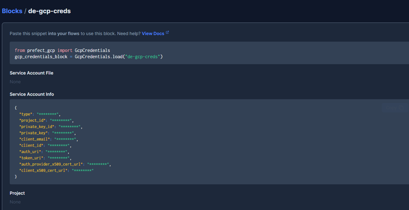
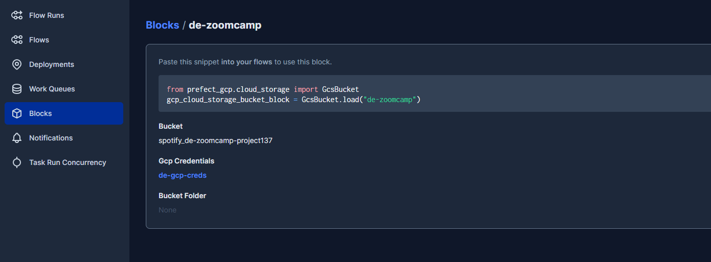
The basic config template is included below for reference :

from prefect_gcp import GcpCredentials
from prefect_gcp.cloud_storage import GcsBucket

# alternative to creating GCP blocks in the UI
# copy your own service_account_info dictionary from the json file you downloaded from google
# IMPORTANT - do not store credentials in a publicly available repository!


credentials_block = GcpCredentials(
    service_account_info={}  # enter your credentials from the json file
)
credentials_block.save("zoom-gcp-creds", overwrite=True)


bucket_block = GcsBucket(
    gcp_credentials=GcpCredentials.load("zoom-gcp-creds"),
    bucket="prefect-de-zoomcamp",  # insert your  GCS bucket name
)

bucket_block.save("zoom-gcs", overwrite=True)

Once you are ready to run your flows you can make use of the Prefect UI to visualise the flows by entering the following at the command line:

prefect orion start

and then navigating to the dashboard at http://127.0.0.1:4200

I created the following Python script to grab the local csv, clean up using pandas, convert to parquet, and upload to Google Cloud Storage. I ran the file from the command line using :

python etl_web_to_gcs.py

etl_web_to_gcs.py

from pathlib import Path
import pandas as pd
from prefect import flow, task
from prefect_gcp.cloud_storage import GcsBucket
import pyarrow as pa
from random import randint


@task(retries=3)
def fetch(dataset_url: str) -> pd.DataFrame:
    """Read data into pandas DataFrame"""
    df = pd.read_csv(dataset_url)
    return df


@task(log_prints=True)
def clean(df: pd.DataFrame) -> pd.DataFrame:
   """Some pandas transforms and print basic info"""
   df = df.drop(['id', 'album_id', 'artist_ids', 'track_number', 'disc_number', 'time_signature'], axis=1)
   df.loc[815351:815360,'year'] = 2018
   df.loc[450071:450076,'year'] = 1996
   df.loc[459980:459987,'year'] = 1991
   df['artists'] = df['artists'].str.strip("['']")
   df['danceability'] = df['danceability'].round(2)
   df['energy'] = df['energy'].round(2)
   df['loudness'] = df['loudness'].round(2)
   df['speechiness'] = df['speechiness'].round(2)
   df['acousticness'] = df['acousticness'].round(2)
   df['instrumentalness'] = df['instrumentalness'].round(2)
   df['liveness'] = df['liveness'].round(2)
   df['valence'] = df['valence'].round(2)
   df["tempo"] = df["tempo"].astype(int)
   df['year_date'] = pd.to_datetime(df['year'], format='%Y')
   df["duration_s"] = (df["duration_ms"] / 1000).astype(int).round(0)

   print(df.head(2))
   print(f"columns: {df.dtypes}")
   print(f"rows: {len(df)}")
   return df


@task()
def write_local(df: pd.DataFrame, dataset_file: str) -> Path:
   """Write DataFrame out locally as parquet file"""
   path = Path(f"data/{dataset_file}.parquet")
   df.to_parquet(path, compression="gzip")
   return path


@task()
def write_gcs(path: Path) -> None:
    """Upload local parquet file to GCS"""
    gcs_block = GcsBucket.load("de-zoomcamp")
    gcs_block.upload_from_path(from_path=path, to_path=path)
    return


@flow()
def etl_web_to_gcs() -> None:
    """The main ETL function"""
    dataset_file = "spotify"
    dataset_url = "data/spotify.csv"
    df = fetch(dataset_url)
    df_clean = clean(df)
    path = write_local(df_clean,dataset_file)
    write_gcs(path)
    
if __name__ == "__main__":
    etl_web_to_gcs()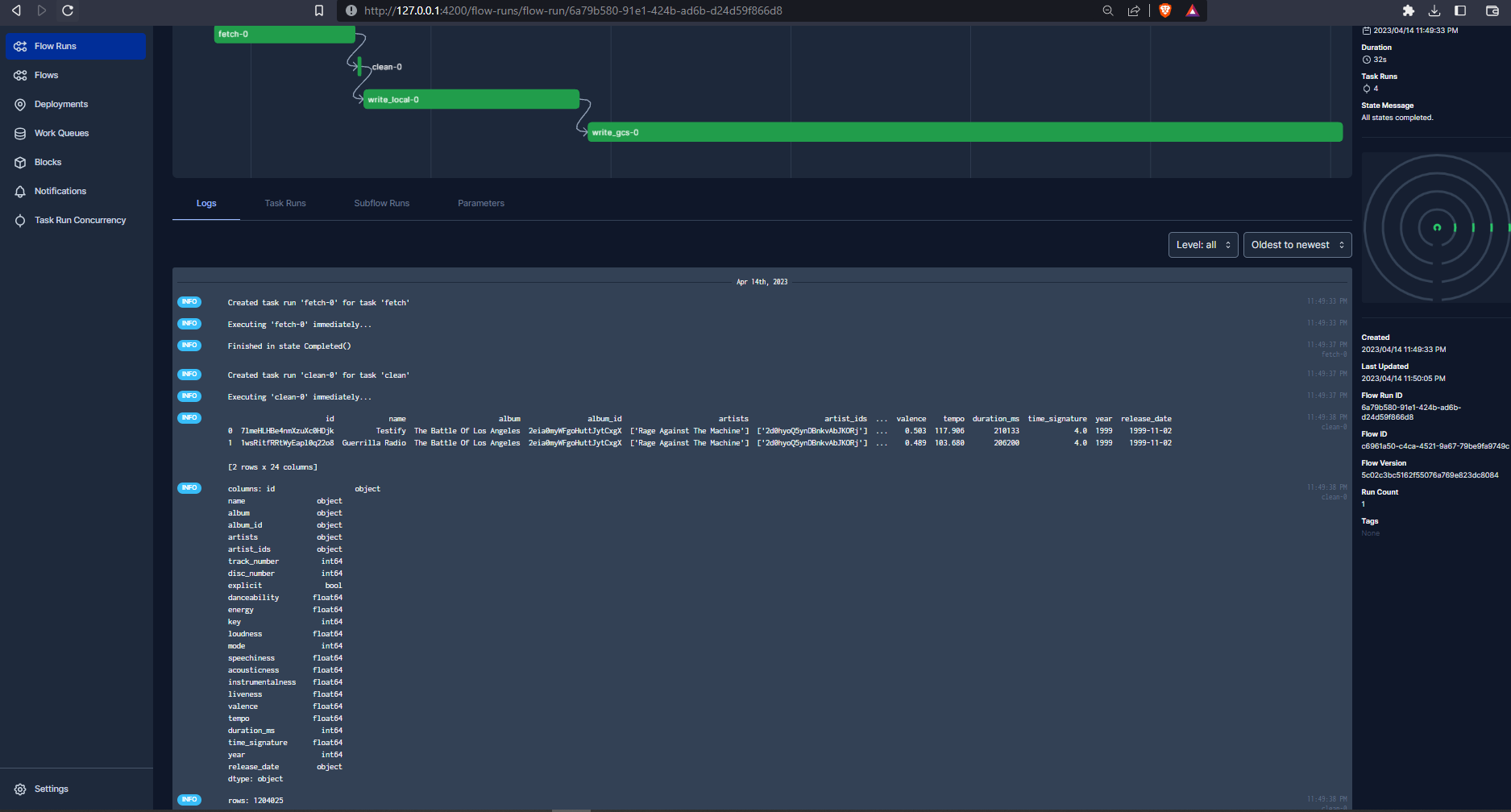

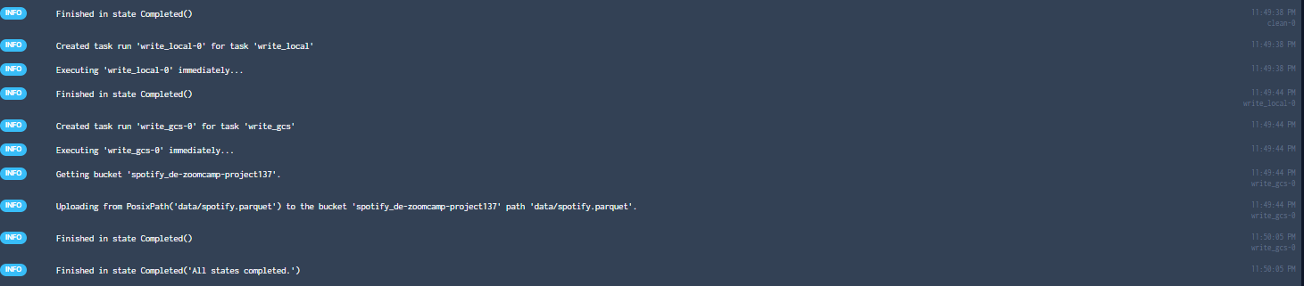
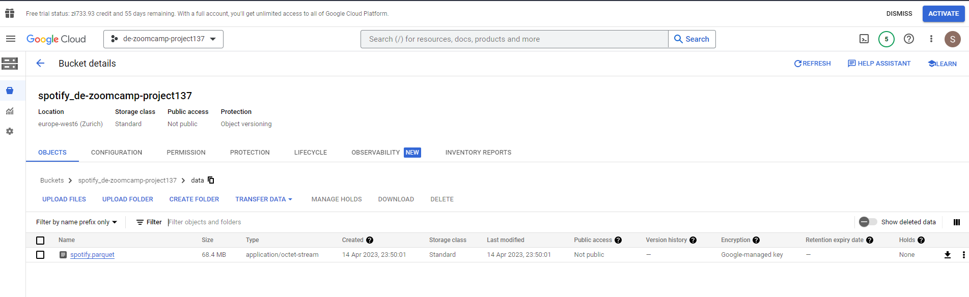
prefect_etl_web_to_gcs_1.PNG

prefect_etl_web_to_gcs_2.PNG

That has completed successfully. The parquet file has been uploaded to our data lake :

bucket.PNG

I created the following Python script to take the parquet file from Google Cloud Storage and write to BigQuery as a table, and ran the file from the command line using :

python etl_web_to_gcs.py

etl_gcs_to_bq.py

from pathlib import Path
import pandas as pd
from prefect import flow, task
from prefect_gcp.cloud_storage import GcsBucket
from prefect_gcp import GcpCredentials


@task(retries=3)
def extract_from_gcs() -> Path:
    """Download data from GCS"""
    gcs_path = Path(f"data/spotify.parquet")
    gcs_block = GcsBucket.load("de-zoomcamp")
    gcs_block.get_directory(from_path=gcs_path, local_path=f"./data/")
    return Path(f"{gcs_path}")

@task()
def transform(path: Path) -> pd.DataFrame:
    """Print some basic info"""
    df = pd.read_parquet(path)
    print(df.head(2))
    print(f"columns: {df.dtypes}")
    print(f"rows: {len(df)}")
    return df
 

@task()
def write_bq(df: pd.DataFrame) -> None:
    """Write DataFrame to BiqQuery"""

    gcp_credentials_block = GcpCredentials.load("de-gcp-creds")

    df.to_gbq(
        destination_table="spotify.spotify_one_point_two_million",
        project_id="de-zoomcamp-project137",
        credentials=gcp_credentials_block.get_credentials_from_service_account(),
        chunksize=500_000,
        if_exists="replace",
    )


@flow()
def etl_gcs_to_bq():
    """Main ETL flow to load data into Big Query"""
    path = extract_from_gcs()
    df = transform(path)
    write_bq(df)


if __name__ == "__main__":
    etl_gcs_to_bq()

prefect_etl_gcs_to_bq.PNG

prefect_etl_gcs_to_bq_1.PNG

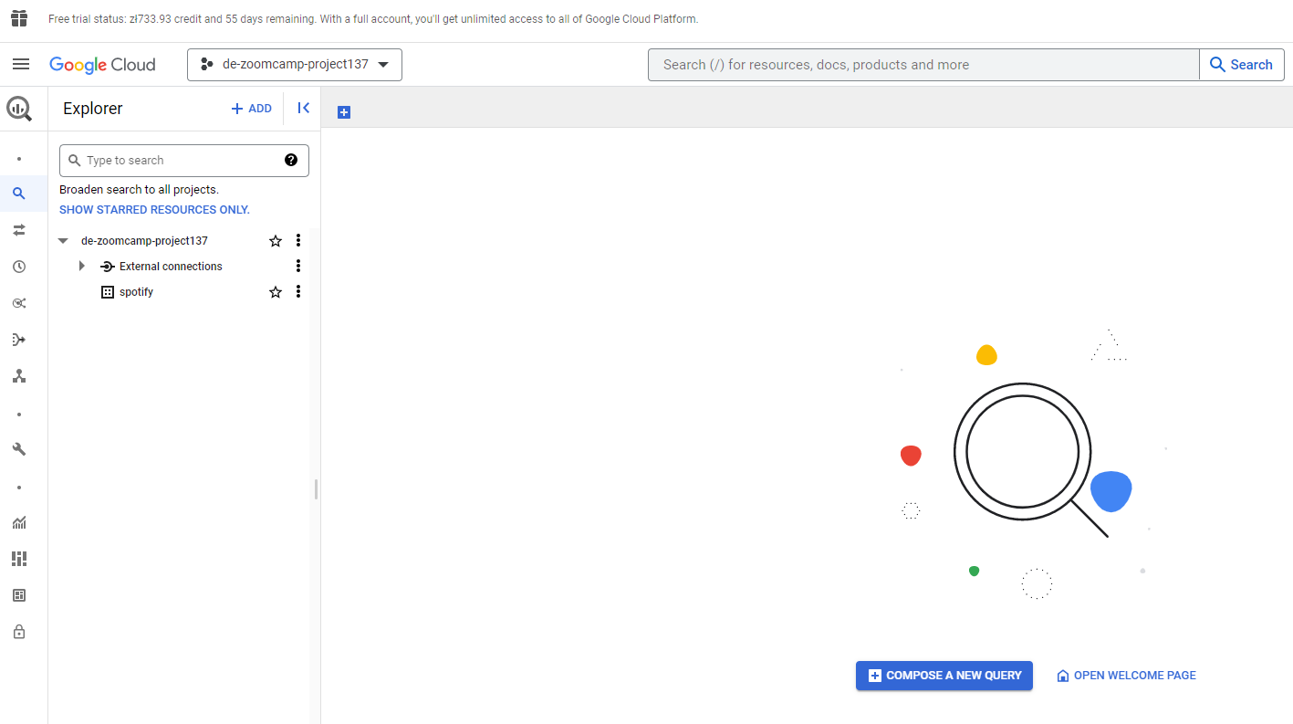
That has also completed successfully. A table has been created in BigQuery from the data held in Google Cloud Storage :

big_query.PNG

4. Data Transformation

Set up dbt cloud within BigQuery

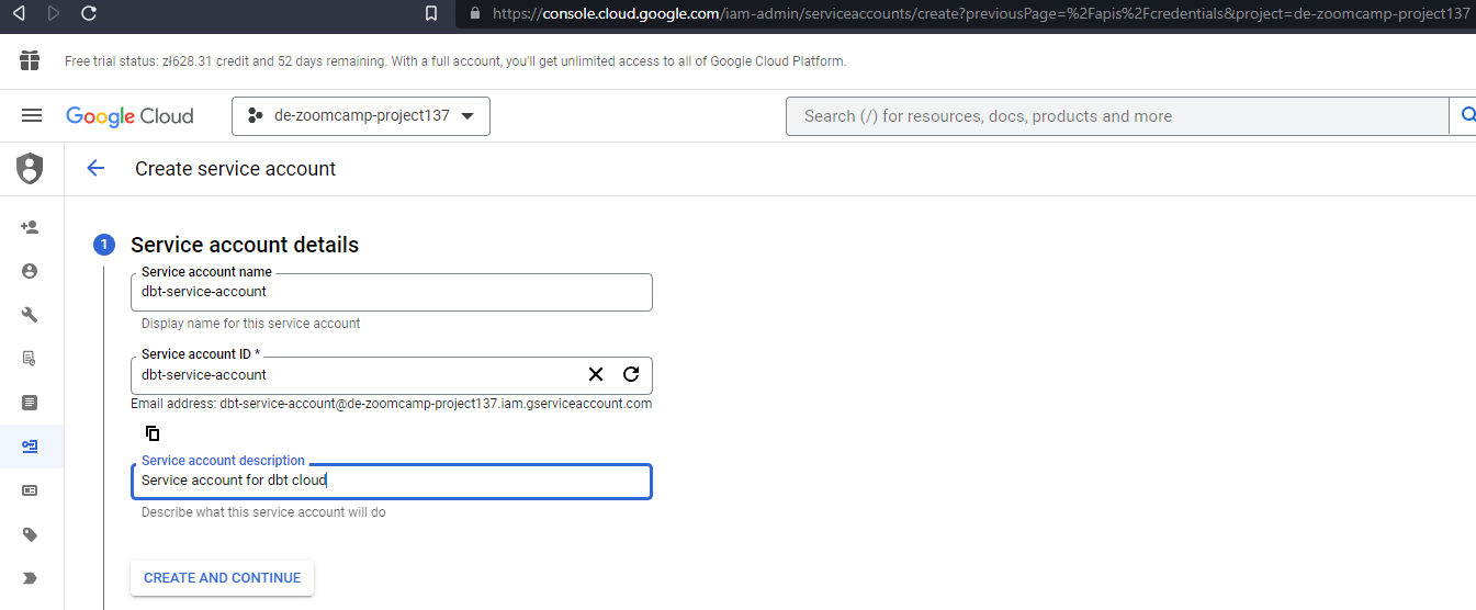
We need to create a dedicated service account within Big Query to enable communication with dbt cloud.

1. Open the BigQuery credential wizard to create a service account in your project :

big_query_dbt.PNG

dbt_service_account.PNG

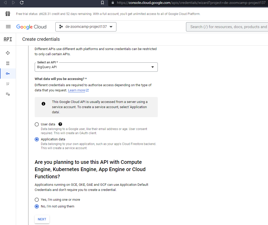
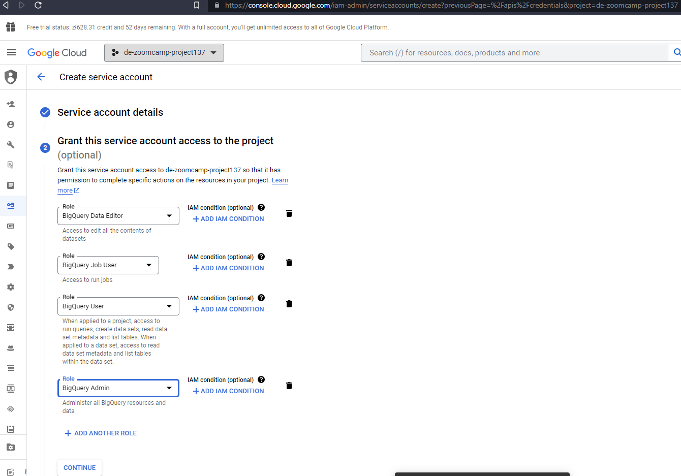
2. You can either grant the specific roles the account will need or simply use BigQuery Admin, as you’ll be the sole user of both accounts and data.

Note: if you decide to use specific roles instead of BQ Admin, some users reported that they needed to add also viewer role to avoid encountering denied access errors.

dbt_service_account_grantaccess.PNG

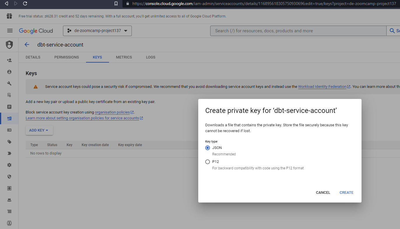
3. Now that the service account has been created we need to add and download a JSON key, go to the keys section, select “create new key”. Select key type JSON and once you click on CREATE it will get inmediately downloaded for you to use.

dbt_service_account_key.PNG

Create a dbt cloud project

1. Create a dbt cloud account from their website (free for freelance developers)
2. Once you have logged in you will be prompted to Complete Project Setup
3. Naming your project - a default name Analytics is given
4. Choose BigQuery as your data warehouse:
5. Upload the key you downloaded from BigQuery. This will populate most fields related to the production credentials.

dbt_project_setup.PNG

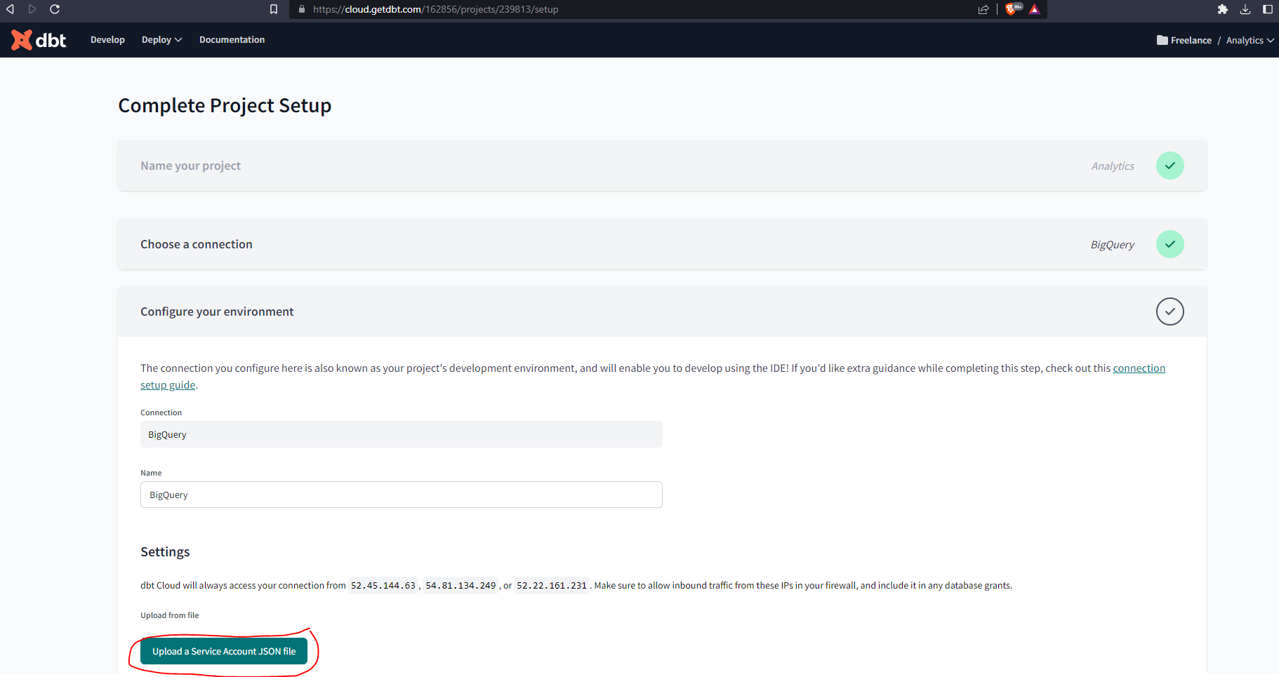
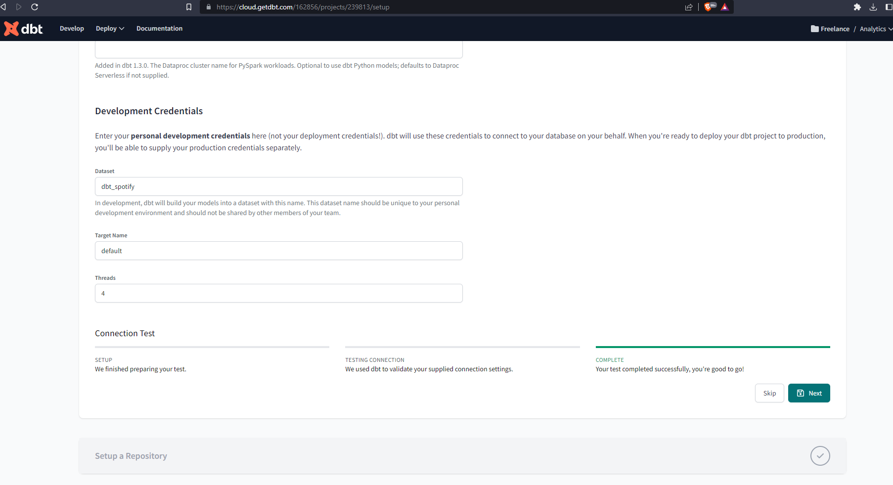
Scroll down to the end of the page, set up your development credentials, and run the connection test and hit Next:

dbt_development_credentials.PNG

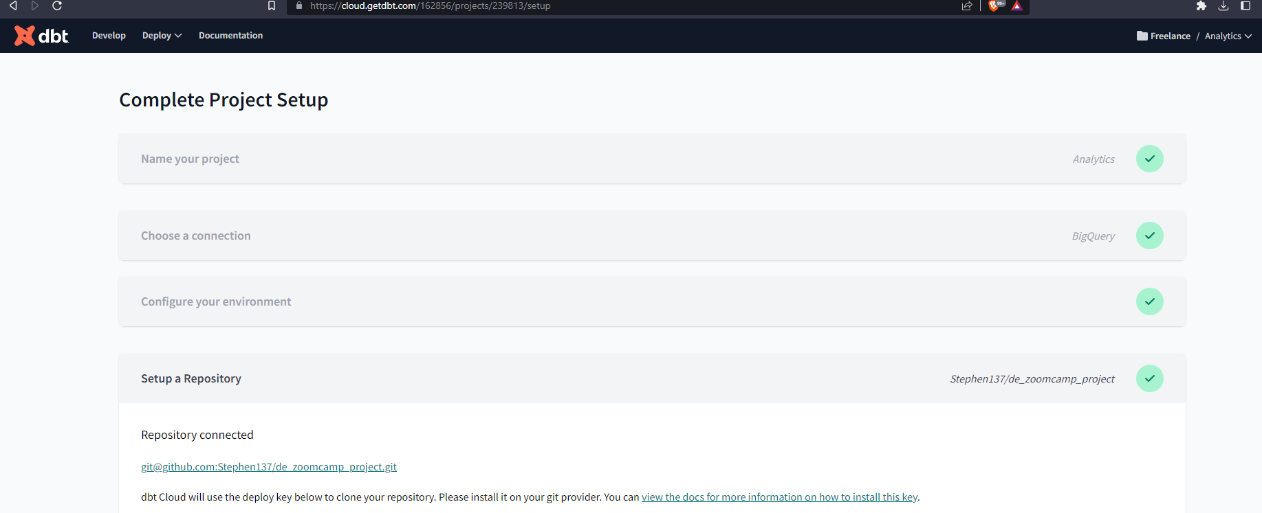
Add GitHub repository

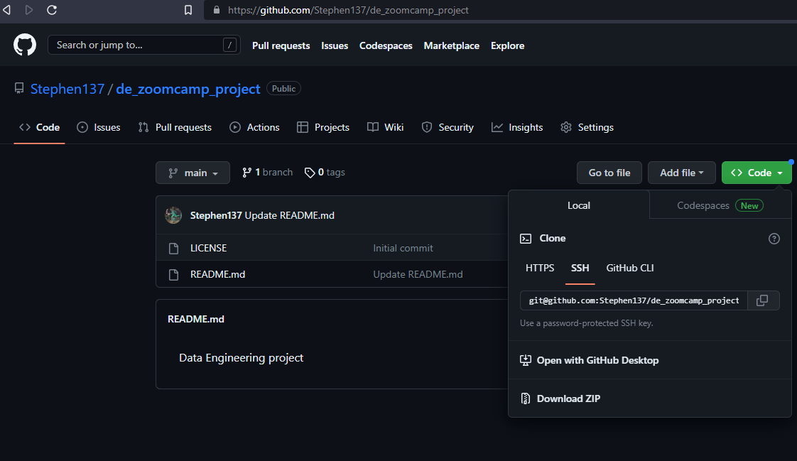
1. Select git clone and paste the SSH key from your repo. Then hit Import

project_github_repo.PNG

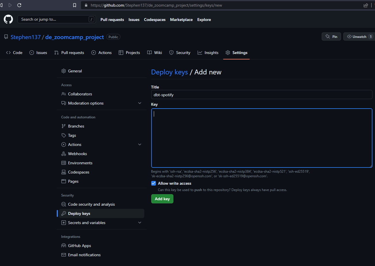
2. You will get a deploy key :

image.png

3. Head to your GH repo and go to the settings tab. Under security you’ll find the menu deploy keys. Click on Add deploy key and paste the deploy key provided by dbt cloud. Make sure to tick on “write access”.

add_dbt_deploy_key_to_github.PNG

For a detailed set up guide see here.

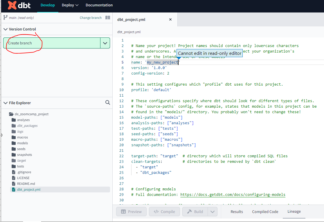
Initialize dbt project

This builds out your folder structure with example models.

Make your initial commit by clicking Commit and sync. Use the commit message “initial commit” and click Commit. Note that the files are read-only and you have to Create branch before you can edit or add new files :

dbt_initial_commit.PNG

Once you have created a branch you can edit and add new files. Essentially we only need three files to build our model :

dbt.project.yml

The basic config below can be tailored to meet your own needs. The key fields are :

name <spotify_dbt> This will be the name of the dataset created in BiqQuery on successful run of the transformation model

models:
<spotify_dbt> This should match the name specified above

# Name your project! Project names should contain only lowercase characters
# and underscores. A good package name should reflect your organization's
# name or the intended use of these models

name: 'spotify_dbt' # This will be the name of the dataset dbt will create in BigQuery
version: '1.0.0'
config-version: 2

# This setting configures which "profile" dbt uses for this project.
profile: 'default'

# These configurations specify where dbt should look for different types of files.
# The `source-paths` config, for example, states that models in this project can be
# found in the "models/" directory. You probably won't need to change these!
model-paths: ["models"]
analysis-paths: ["analyses"]
test-paths: ["tests"]
seed-paths: ["seeds"]
macro-paths: ["macros"]
snapshot-paths: ["snapshots"]

target-path: "target"  # directory which will store compiled SQL files
clean-targets:         # directories to be removed by `dbt clean`
  - "target"
  - "dbt_packages"


# Configuring models
# Full documentation: https://docs.getdbt.com/docs/configuring-models

# In this example config, we tell dbt to build all models in the example/ directory
# as tables. These settings can be overridden in the individual model files
# using the `{{ config(...) }}` macro.
models:
  spotify_dbt:
      # Applies to all files under models/.../
      staging:
          materialized: view

schema.yml

Note that this file also includes the source i.e. the location of the data that the transforms included in our model are to be performed on :

name : <spotify> Choose a name for this source variable, This will be referenced in the model.sql file
database: <de-zoomcamp-project137> BigQuery project reference

version: 2

sources:
    - name: spotify # Choose a name. This will be the 'source' referred to in the 
      database: de-zoomcamp-project137 # BigQuery project reference
      tables:
        - name: spotify_one_point_two_million # Choose a name for the table to be created in BigQuery
       
models:
    - name: spotify_one_point_two_million
      description: >
        Curated by Rodolfo Gigueroa, over 1.2 million songs downloaded from the MusicBrainz catalog and 24 track features obtained using the Spotify
        API. 
      columns:
          - name: id
            description: >
              The base-62 identifier found at the end of the Spotify URI for an artist, track, album, playlist, etc. Unlike a Spotify URI, a Spotify ID
              does not clearly identify the type of resource; that information is provided elsewhere in the call. 
          - name: name 
            description: The name of the track                         
          - name: album
            description: The name of the album. In case of an album takedown, the value may be an empty string.
          - name: album_id
            description: The Spotify ID for the album.
          - name: artists
            description: The name(s) of the artist(s).
          - name: artist_ids
            description: The Spotify ID for the artist(s).
          - name: track_number
            description: The number of the track. If an album has several discs, the track number is the number on the specified disc.
          - name: disc_number
            description: The disc number (usually 1 unless the album consists of more than one disc).
          - name: explicit
            description: Whether or not the track has explicit lyrics ( true = yes it does; false = no it does not OR unknown).
          - name: danceability
            description: >
             Danceability describes how suitable a track is for dancing based on a combination of musical elements including tempo, rhythm stability, 
             beat strength, and overall regularity. A value of 0.0 is least danceable and 1.0 is most danceable.           
          - name: energy 
            description: >
             Energy is a measure from 0.0 to 1.0 and represents a perceptual measure of intensity and activity. Typically, energetic tracks feel fast,
             loud, and noisy. For example, death metal has high energy, while a Bach prelude scores low on the scale. Perceptual features contributing
             to this attribute include dynamic range, perceived loudness, timbre, onset rate, and general entropy.
          - name: key
            description: >
             The key the track is in. Integers map to pitches using standard Pitch Class notation. E.g. 0 = C, 1 = C♯/D♭, 2 = D, and so on. If no key 
             was detected, the value is -1.
          - name: loudness
            description: >
             The overall loudness of a track in decibels (dB). Loudness values are averaged across the entire track and are useful for comparing 
             relative loudness of tracks. Loudness is the quality of a sound that is the primary psychological correlate of physical strength 
             (amplitude). Values typically range between -60 and 0 db.
          - name: mode
            description: >
              Mode indicates the modality (major or minor) of a track, the type of scale from which its melodic content is derived. Major is represented
              by 1 and minor is 0.
          - name: speechiness
            description: >
              Speechiness detects the presence of spoken words in a track. The more exclusively speech-like the recording (e.g. talk show, audio book, 
              poetry), the closer to 1.0 the attribute value. Values above 0.66 describe tracks that are probably made entirely of spoken words. Values 
              between 0.33 and 0.66 describe tracks that may contain both music and speech, either in sections or layered, including such cases as rap 
              music. Values below 0.33 most likely represent music and other non-speech-like tracks.         
          - name: acousticness
            description: A confidence measure from 0.0 to 1.0 of whether the track is acoustic. 1.0 represents high confidence the track is acoustic.
          - name: instrumentalness
            description: >
             Predicts whether a track contains no vocals. "Ooh" and "aah" sounds are treated as instrumental in this context. Rap or spoken word tracks 
             are clearly "vocal". The closer the instrumentalness value is to 1.0, the greater likelihood the track contains no vocal content. Values above 
             0.5 are intended to represent instrumental tracks, but confidence is higher as the value approaches 1.0.
          - name: liveness
            description: >
             Detects the presence of an audience in the recording. Higher liveness values represent an increased probability that the track was performed 
             live. A value above 0.8 provides strong likelihood that the track is live.
          - name: valence
            description: A measure from 0.0 to 1.0 describing the musical positiveness conveyed by a track. Tracks with high valence sound more positive (e.g. happy, cheerful, euphoric), while tracks with low valence sound more negative (e.g. sad, depressed, angry).
          - name: tempo
            description: >
             The overall estimated tempo of a track in beats per minute (BPM). In musical terminology, tempo is the speed or pace of a given piece and 
             derives directly from the average beat duration.
          - name: duration_ms
            description: The duration of the track in milliseconds.
          - name: time_signature
            description: >
             An estimated time signature. The time signature (meter) is a notational convention to specify how many beats are in each bar (or measure). 
             The time signature ranges from 3 to 7 indicating time signatures of "3/4", to "7/4".
          - name: year
            description: The year in which the track was released
          - name: release_date
            description: Release date of the track in the format 2023-04-17

spotify_one_point_two_million.sql

Although this is a .sql file this is actually our transformation model. Note the first line configuration overrides the materialized setting that I configured in my dbt.project.yml file.

Note also the following :

FROM {{ source('spotify', 'spotify_one_point_two_million')}}

This specifies that dbt will apply transformations on my dataset in BiqQuery named spotify and specifically, on the table named spotify_one_point_two_million.

{{ config(materialized='table') }}

SELECT 
    -- identifiers
    name,
    album,
    artists,
    explicit,
    danceability,
    energy,
    {{ get_key_description('key') }} AS key_description, 
    loudness,
    {{ get_modality_description('mode') }} AS modality_description, 
    speechiness,
    acousticness,
    instrumentalness,
    liveness,
    valence,
    tempo,
    duration_s,
    year_date,
     CASE
        WHEN year_date BETWEEN '1900-01-01 00:00:00 UTC' AND '1909-12-31 00:00:00 UTC' THEN 'Naughts'
        WHEN year_date BETWEEN '1910-01-01 00:00:00 UTC' AND '1919-12-31 00:00:00 UTC' THEN 'Tens'
        WHEN year_date BETWEEN '1920-01-01 00:00:00 UTC' AND '1929-12-31 00:00:00 UTC' THEN 'Roaring Twenties'
        WHEN year_date BETWEEN '1930-01-01 00:00:00 UTC' AND '1939-12-31 00:00:00 UTC' THEN 'Dirty Thirties'
        WHEN year_date BETWEEN '1940-01-01 00:00:00 UTC' AND '1949-12-31 00:00:00 UTC' THEN 'Forties'
        WHEN year_date BETWEEN '1950-01-01 00:00:00 UTC' AND '1959-12-31 00:00:00 UTC' THEN 'Fabulous Fifties'
        WHEN year_date BETWEEN '1960-01-01 00:00:00 UTC' AND '1969-12-31 00:00:00 UTC' THEN 'Swinging Sixties'
        WHEN year_date BETWEEN '1970-01-01 00:00:00 UTC' AND '1979-12-31 00:00:00 UTC' THEN 'Seventies'
        WHEN year_date BETWEEN '1980-01-01 00:00:00 UTC' AND '1989-12-31 00:00:00 UTC' THEN 'Eighties'
        WHEN year_date BETWEEN '1990-01-01 00:00:00 UTC' AND '1999-12-31 00:00:00 UTC' THEN 'Nineties'
        WHEN year_date BETWEEN '2000-01-01 00:00:00 UTC' AND '2009-12-31 00:00:00 UTC' THEN 'Noughties'
        WHEN year_date BETWEEN '2010-01-01 00:00:00 UTC' AND '2019-12-31 00:00:00 UTC' THEN 'Teens'
        WHEN year_date = '2020-01-01 00:00:00 UTC' THEN '2020'
    END AS Decade,
    CASE
        WHEN valence > 0.5 THEN 'Happy'
        WHEN valence < 0.5 THEN 'Sad'
        ELSE 'Ambivalent'
    END AS Happy_Sad
        
FROM {{ source('spotify', 'spotify_one_point_two_million')}}

You might wonder what this syntax is :

{{ get_key_description('key') }} AS key_description, 

Macros in Jinja are pieces of code that can be reused multiple times – they are analogous to “functions” in other programming languages, and are extremely useful if you find yourself repeating code across multiple models. Macros are defined in .sql files :

get_key_description

 {#
    This macro returns the description of the key
#}

{% macro get_key_description(key) -%}

    case {{ key }}
        when 0 then 'C'
        when 1 then 'C#'
        when 2 then 'D'
        when 3 then 'D#'
        when 4 then 'E'
        when 5 then 'F'
        when 6 then 'F#'
        when 7 then 'G'
        when 8 then 'G#'
        when 9 then 'A'
        when 10 then 'A#'
        when 11 then 'B'

    end

{%- endmacro %}

get_modality_description

 {#
    This macro returns the description of the modality
#}

{% macro get_modality_description(mode) -%}

    case {{ mode }}
        when 0 then 'Minor'
        when 1 then 'Major'
       
    end

{%- endmacro %}

Now that we have our files set up we are ready to run our model. We can see from the lineage that all the connections are complete :

dbt_lineage.PNG

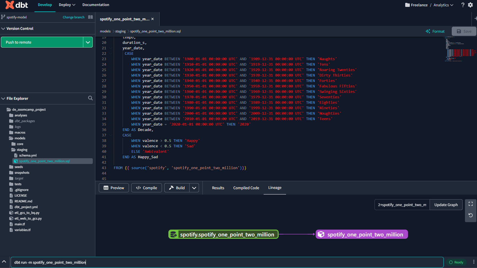
We can run the model from the dbt console using :

dbt run -m <model_name.sql>

And we can see from the system log that the run was successful :

dbt_system_log.PNG

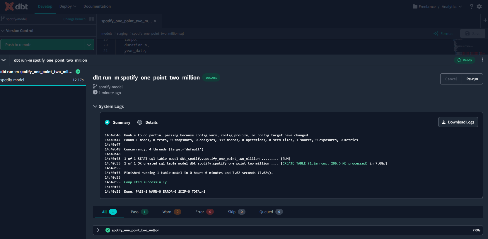
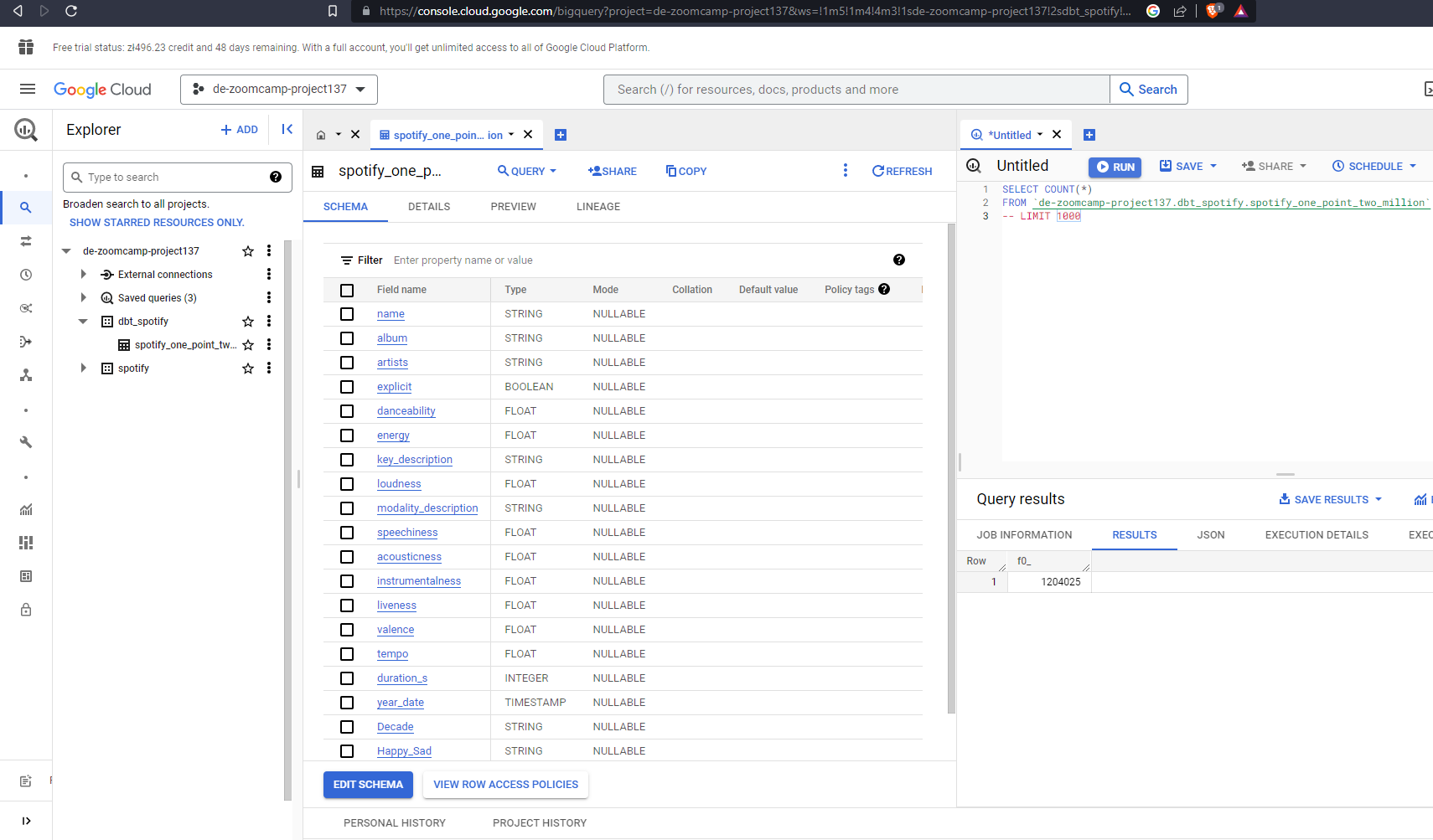
And we have our table created in Big Query with 1,204,025 rows as expected.

biq_query_table.PNG

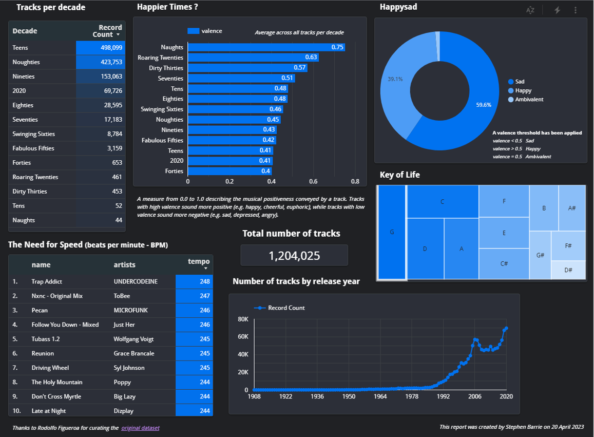
5. Visualization

We’ve come a long way since downloading our raw csv file from Kaggle. Our journey is almost over. It’s time now to visualize our data and gather some insights. For this purpose I will be using Looker Studio. This will allow us to connect to our newly created table in BigQuery and create a Dashboard.

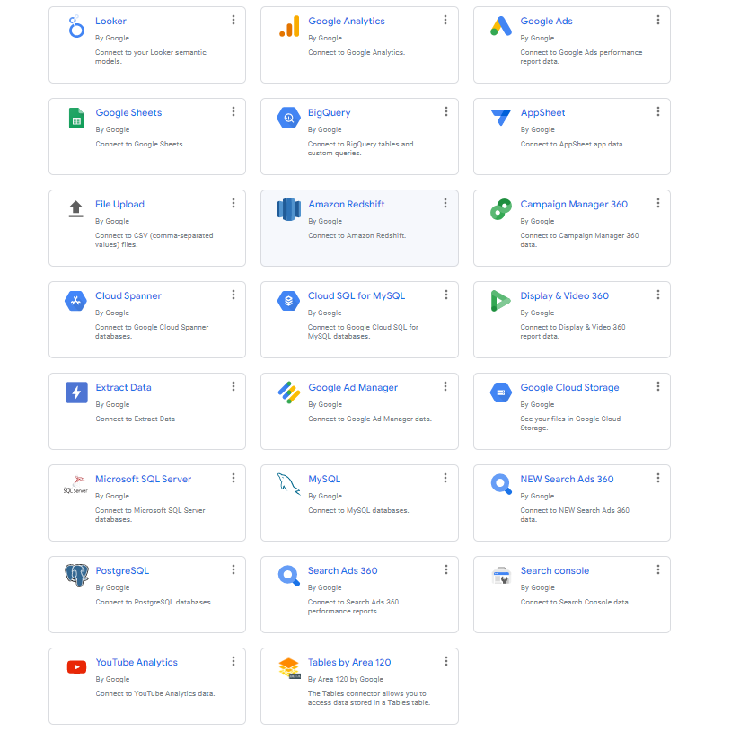
The first thing we need to do is create a data source. There are 23 different connectors at the time of writing. We will be using BigQuery :

looker_connectors.PNG

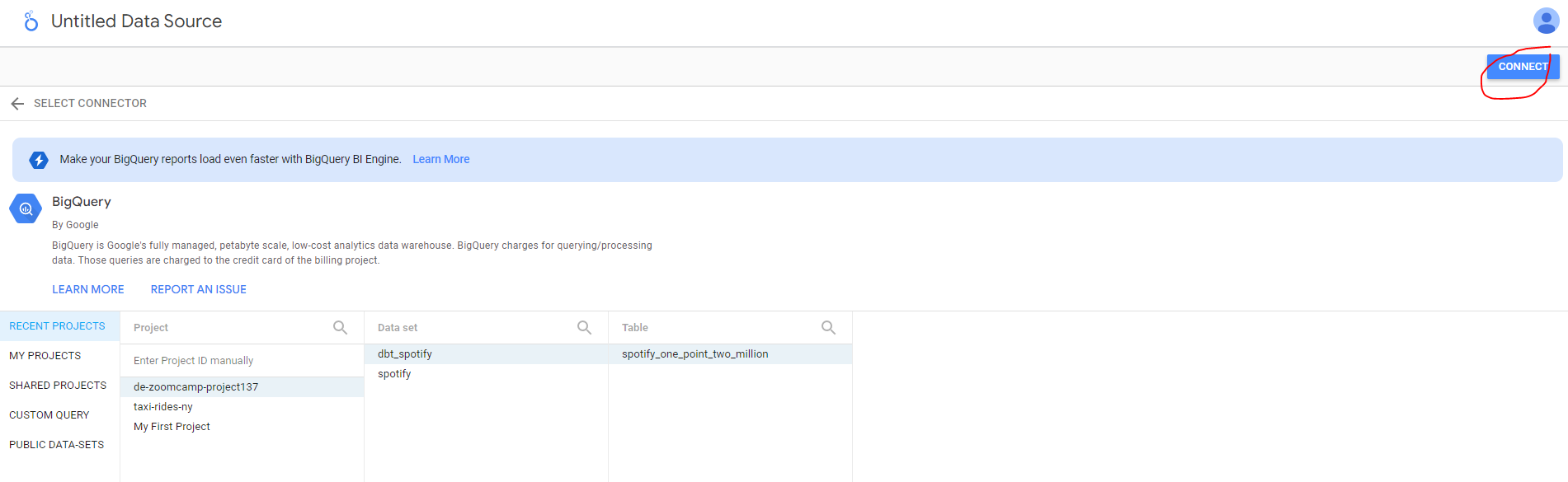
Our recent dataset and table are sitting there ready for connection :

looker_dataset.PNG

Hit CONNECT and we see our fields or columns are there with default settings attached which can be modified if required. Finally hit CREATE REPORT and you are taken to a blank canvass dashboard where the magic begins :)

blank_canvass.PNG

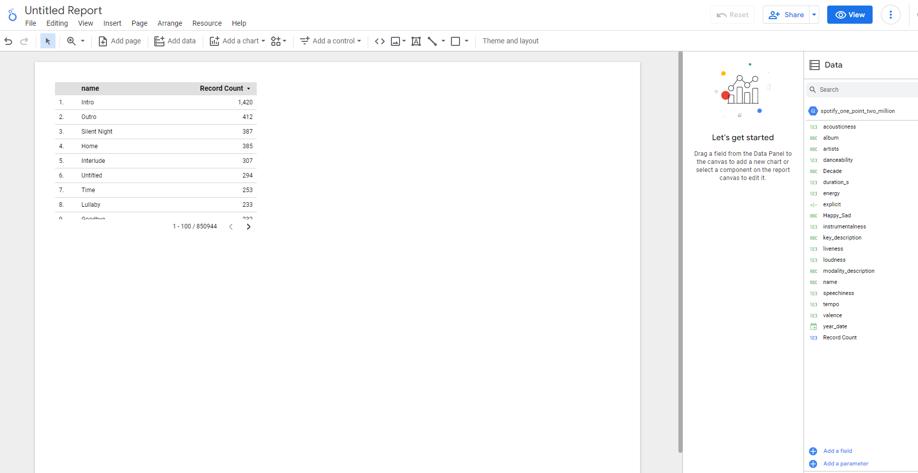
For a complete guide you can check out the Looker Documentation, but the console is very intuitive, and a few strokes of the brush (or clicks of the keyboard) and I was able to produce this dashboard (screenshot included below if you can’t access the link).

Looker.PNG