Into the Unknown - Data Engineering Zoomcamp

Week 1 - Basics and Set-up

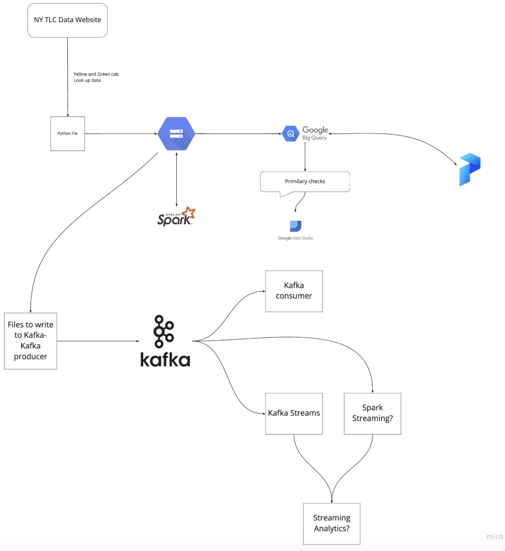
This course will cover a number of technologies, including Google Cloud Platform (GCP): Cloud-based auto-scaling platform by Google, Google Cloud Storage (GCS): Data Lake, BigQuery: Data Warehouse, Terraform: Infrastructure-as-Code (IaC), Docker: Containerization, SQL: Data Analysis & Exploration, Prefect: Workflow Orchestration, dbt: Data Transformation, Spark: Distributed Processing, Kafka: Streaming.

An overview of the course architecture is included below:

The first thing to do is to navigate to the course github page and clone the course repo to your local machine :

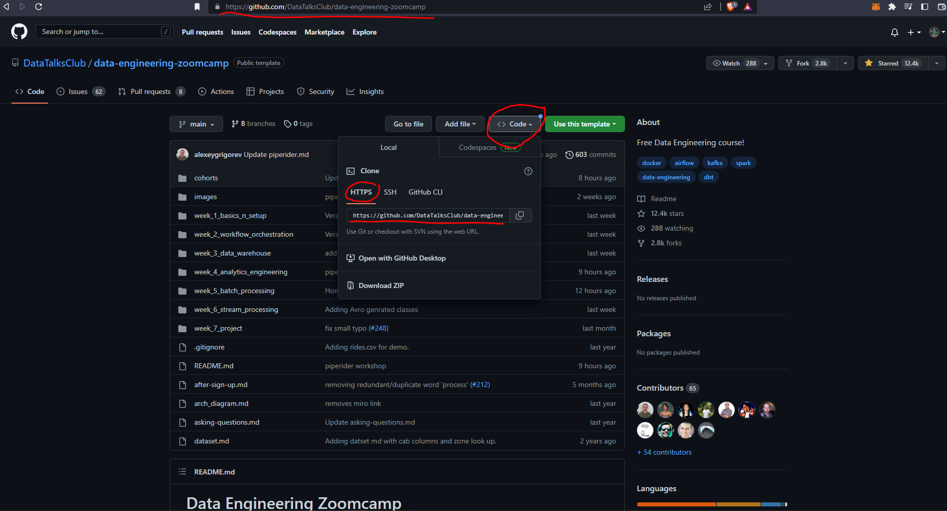
by running the following command in your terminal. I have a Windows machine but have a Linux environment installed, and use the Ubuntu on Windows terminal.

git clone https://github.com/DataTalksClub/data-engineering-zoomcamp.git

I have a nifty terminal splitter called tmux which allows me to have multiple terminals running - which comes in very handy sometimes!!! There’s a handy cheatsheet here but basically CTRL+B is the way in to the magic :)

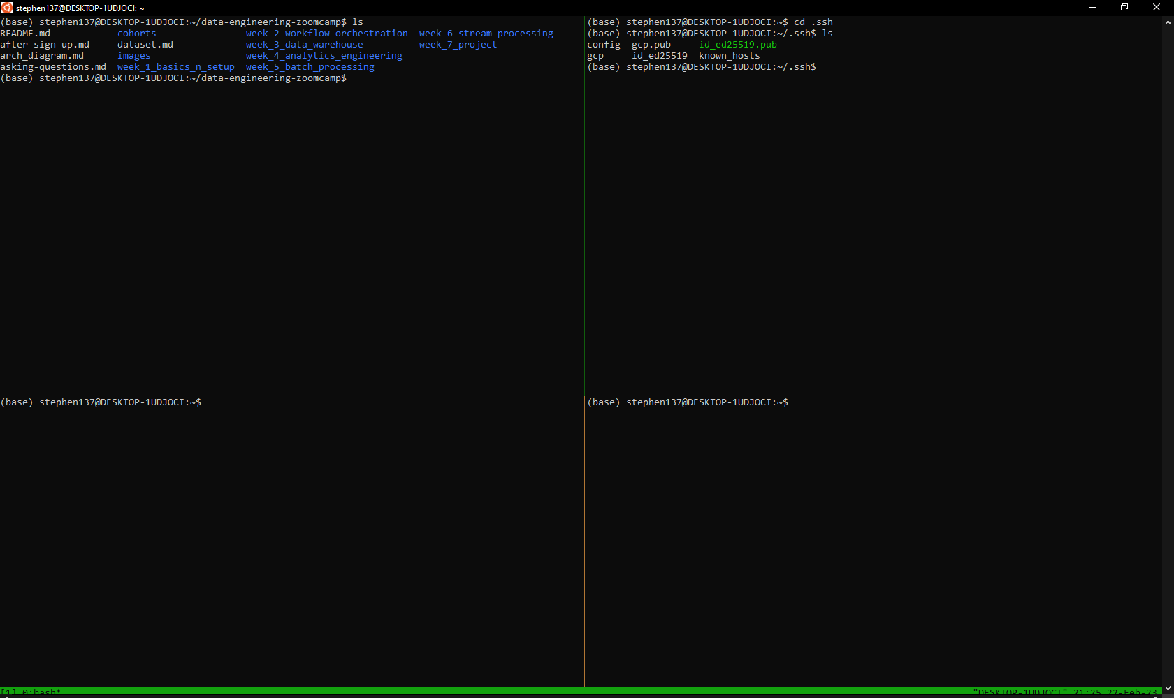
Other things we can do from the command line:

ls (lists all files in the directory)
exit (self explanatory)
rm -rf / (remove all files from directory)

We can use sudo to execute commands where we don’t have the necessary permissions.

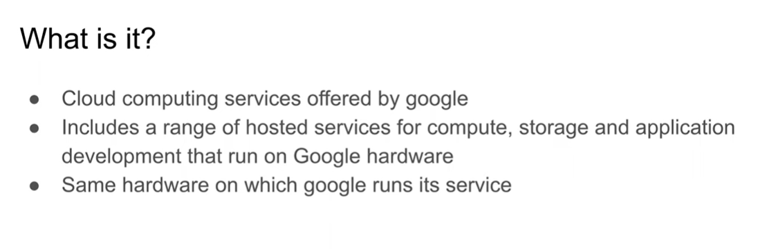
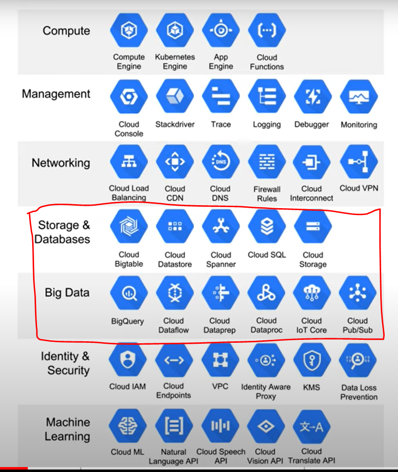
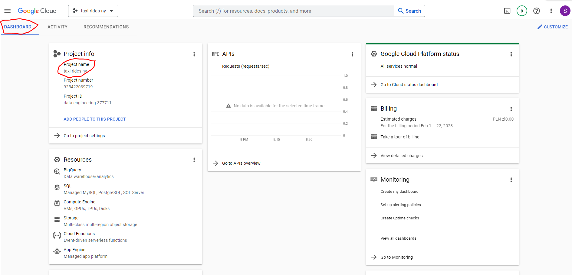
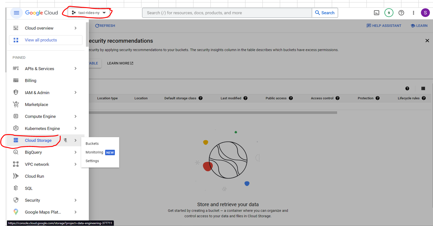
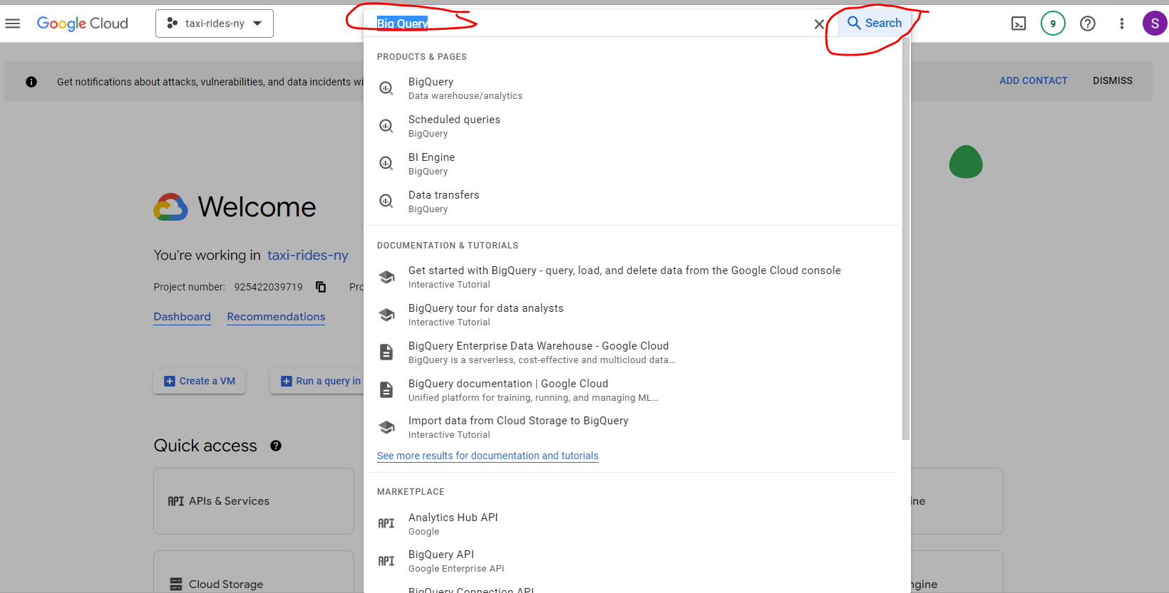
1.1.1 Introduction to Google Cloud Platform (GCP)

1.2.1 Introduction to Docker

What is Docker? Why do we need it?

Docker is an open platform for developing, shipping, and running applications. Docker enables you to separate your applications from your infrastructure so you can deliver software quickly. With Docker, you can manage your infrastructure in the same ways you manage your applications. By taking advantage of Docker’s methodologies for shipping, testing, and deploying code quickly, you can significantly reduce the delay between writing code and running it in production.

You can find out more from the source documentation.

Local experiments
Integration tests (Continuous Integraton (CI) / Continuous Development (CD)) - Github Actions, Jenkins
Reproducibility (isolated CONTAINER) ensures environment on local machine can be directly replicated ANYWHERE
Running pipelines on the cloud (AWS Batch, Kubernetes jobs)
Spark
Serverless (AWS Lambda, [Google] Cloud functions)

Let’s illustrate how Docker works with a simple example. First let’s create a Dockerfile within Visual Studio Code (VSC). VSC can be accessed from the command line using :

code .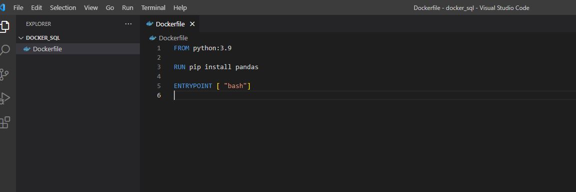

Let’s first build an image - we’ll name it test:pandas by running the following command from within the terminal:

docker build -t test:pandas . # this searches in the current directory for a dockerfile and creates an image

and run the image using :

docker run -it test:pandas

This takes us to a bash command prompt, as this is our entrypoint as defined in our Dockerfile. We can then open up Python, import pandas and check which version we have:

python
import pandas as pd
pd.__version__

The key point about images is that they are as the name suggests a snapshot of all file dependencies at the specific point in time that they are created.

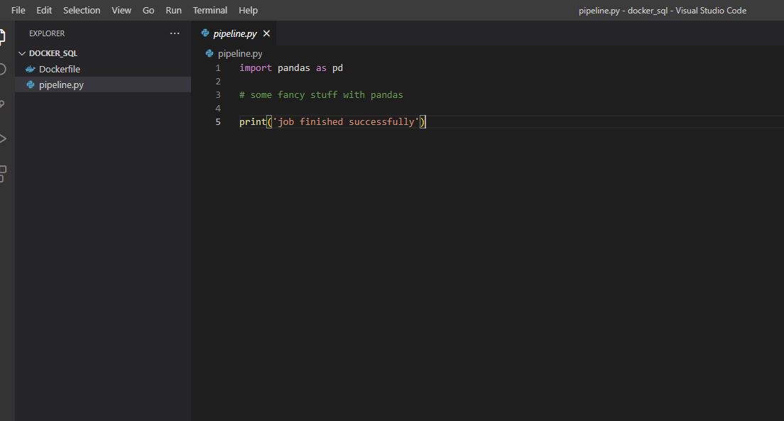
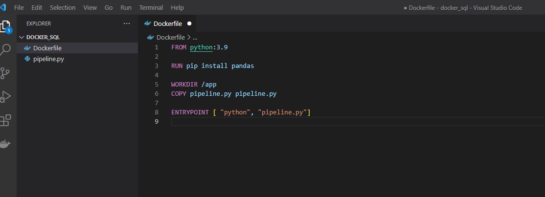
We can automate things further by creating a data pipeline.py file and configuring our Dockerfile to include this :

Let’s run the following commands in the terminal :

docker build -t test:pandas .
docker run -it test:pandas


root@f009333fb3e5:/app# pwd (`pwd` takes us to the CURRENT directory)
/app

We can see that this is /app as specified in WORKDIR in our Dockefile above. Finally, if we run our pipeline.py file:

python pipeline.py

we get the following output:

job finished successfully

This was the final item in our pipeline.py file :)

Fine tuning our Docker container

Let’s fine tune the configuration of our pipleline a bit more prior to scheduling a run:

We first rebuild using our usual command:

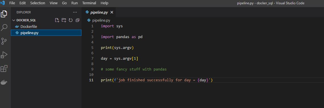
docker build -t test:pandas .

Say we want to schedule the run for a particular today - for illustrative purposes let’s use today’s date. We define day as system argument number 1 (argument 0 is the file name). We then pass in that argument (today’s date - 2023-03-05) in our command line prompt:

docker run -it test:pandas 2023-03-05

And we get the following output:

[‘pipeline.py’, ‘2023-03-05’]

job finished successfully for day = 2023-03-05

The items inside [ ] are the arguments - number 0 is the file name pipeline.py, number 1 is the date as configured in our pipepline. We can include further arguments within our command line prompt e.g :

docker run -it test:pandas 2023-02-09 Incoming_137_new_album!

This returns the following output:

[‘pipeline.py’, ‘2023-02-09’, ‘Incoming.’, ‘137’, ‘new’, ‘album!’] job finished successfully for day = 2023-02-09

The additonal arguments specified are listed as we included

print(sys.arg)

in our pipeline.py file

1.2.2 Ingesting NY Taxi Data to Postgres

Downloading our datasets

Let’s now go ahead and download the datasets that we will be working with over the next few weeks. We can do this from the command line using :

wget https://github.com/DataTalksClub/nyc-tlc-data/releases/download/yellow/yellow_tripdata_2021-01.csv.gz 

wget https://s3.amazonaws.com/nyc-tlc/misc/taxi+_zone_lookup.csv

We can unzip the .gz file and retain the original using :

gzip -dk <file_name.csv.gz>

We can count number of lines using wc (word count) -l (lines) :

wc -l <file_name>

We can look at say the first 100 rows:

head -n 100 <file_name>

We can then save this subset to csv using :

head -n 100 yellow_tripdata_2021-01.csv > yellow_head.csv

We can copy a file to the current directory using :

cp ~ </existing/file/path> .

We can look at a text data file from the command line using:

less <file_name>

and exit the terminal using CTRL + Z

Explore our dataset

Let’s now take a look at our data within Jupter Notebooks using pandas. We will only carry out limited pre-processing at this stage - the focus is to demonstrate how to take a csv file and ingest it to a database.

import pandas as pd

pd.__version__

'1.5.2'

df = pd.read_csv('Data/yellow_tripdata_2021-01.csv')
df

/tmp/ipykernel_194/843851997.py:1: DtypeWarning: Columns (6) have mixed types. Specify dtype option on import or set low_memory=False.
  df = pd.read_csv('Data/yellow_tripdata_2021-01.csv')

	VendorID	tpep_pickup_datetime	tpep_dropoff_datetime	passenger_count	trip_distance	RatecodeID	store_and_fwd_flag	PULocationID	DOLocationID	payment_type	fare_amount	extra	mta_tax	tip_amount	tolls_amount	improvement_surcharge	total_amount	congestion_surcharge
0	1.0	2021-01-01 00:30:10	2021-01-01 00:36:12	1.0	2.10	1.0	N	142	43	2.0	8.00	3.00	0.5	0.00	0.0	0.3	11.80	2.5
1	1.0	2021-01-01 00:51:20	2021-01-01 00:52:19	1.0	0.20	1.0	N	238	151	2.0	3.00	0.50	0.5	0.00	0.0	0.3	4.30	0.0
2	1.0	2021-01-01 00:43:30	2021-01-01 01:11:06	1.0	14.70	1.0	N	132	165	1.0	42.00	0.50	0.5	8.65	0.0	0.3	51.95	0.0
3	1.0	2021-01-01 00:15:48	2021-01-01 00:31:01	0.0	10.60	1.0	N	138	132	1.0	29.00	0.50	0.5	6.05	0.0	0.3	36.35	0.0
4	2.0	2021-01-01 00:31:49	2021-01-01 00:48:21	1.0	4.94	1.0	N	68	33	1.0	16.50	0.50	0.5	4.06	0.0	0.3	24.36	2.5
...	...	...	...	...	...	...	...	...	...	...	...	...	...	...	...	...	...	...
1369760	NaN	2021-01-25 08:32:04	2021-01-25 08:49:32	NaN	8.80	NaN	NaN	135	82	NaN	21.84	2.75	0.5	0.00	0.0	0.3	25.39	0.0
1369761	NaN	2021-01-25 08:34:00	2021-01-25 09:04:00	NaN	5.86	NaN	NaN	42	161	NaN	26.67	2.75	0.5	0.00	0.0	0.3	30.22	0.0
1369762	NaN	2021-01-25 08:37:00	2021-01-25 08:53:00	NaN	4.45	NaN	NaN	14	106	NaN	25.29	2.75	0.5	0.00	0.0	0.3	28.84	0.0
1369763	NaN	2021-01-25 08:28:00	2021-01-25 08:50:00	NaN	10.04	NaN	NaN	175	216	NaN	28.24	2.75	0.5	0.00	0.0	0.3	31.79	0.0
1369764	NaN	2021-01-25 08:38:00	2021-01-25 08:50:00	NaN	4.93	NaN	NaN	248	168	NaN	20.76	2.75	0.5	0.00	0.0	0.3	24.31	0.0

1369765 rows × 18 columns

df.dtypes

VendorID                 float64
tpep_pickup_datetime      object
tpep_dropoff_datetime     object
passenger_count          float64
trip_distance            float64
RatecodeID               float64
store_and_fwd_flag        object
PULocationID               int64
DOLocationID               int64
payment_type             float64
fare_amount              float64
extra                    float64
mta_tax                  float64
tip_amount               float64
tolls_amount             float64
improvement_surcharge    float64
total_amount             float64
congestion_surcharge     float64
dtype: object

Generate table Schema

To generate a schema for use within postgreSQL there is a module within pandas named io to convert to Data Definition Language (DDL) :

print(pd.io.sql.get_schema(df, name='yellow_taxi_data')) # name of Table

CREATE TABLE "yellow_taxi_data" (
"VendorID" REAL,
  "tpep_pickup_datetime" TEXT,
  "tpep_dropoff_datetime" TEXT,
  "passenger_count" REAL,
  "trip_distance" REAL,
  "RatecodeID" REAL,
  "store_and_fwd_flag" TEXT,
  "PULocationID" INTEGER,
  "DOLocationID" INTEGER,
  "payment_type" REAL,
  "fare_amount" REAL,
  "extra" REAL,
  "mta_tax" REAL,
  "tip_amount" REAL,
  "tolls_amount" REAL,
  "improvement_surcharge" REAL,
  "total_amount" REAL,
  "congestion_surcharge" REAL
)

We can see immmediately that pick up and drop off datatype is TEXT but needs to be converted (parsed) to datetime. We can do this using pandas to_datetime:

pd.to_datetime(df.tpep_pickup_datetime)

0         2021-01-01 00:30:10
1         2021-01-01 00:51:20
2         2021-01-01 00:43:30
3         2021-01-01 00:15:48
4         2021-01-01 00:31:49
                  ...        
1369760   2021-01-25 08:32:04
1369761   2021-01-25 08:34:00
1369762   2021-01-25 08:37:00
1369763   2021-01-25 08:28:00
1369764   2021-01-25 08:38:00
Name: tpep_pickup_datetime, Length: 1369765, dtype: datetime64[ns]

pd.to_datetime(df.tpep_dropoff_datetime)

0         2021-01-01 00:36:12
1         2021-01-01 00:52:19
2         2021-01-01 01:11:06
3         2021-01-01 00:31:01
4         2021-01-01 00:48:21
                  ...        
1369760   2021-01-25 08:49:32
1369761   2021-01-25 09:04:00
1369762   2021-01-25 08:53:00
1369763   2021-01-25 08:50:00
1369764   2021-01-25 08:50:00
Name: tpep_dropoff_datetime, Length: 1369765, dtype: datetime64[ns]

We now need to update our dataframe:

df.tpep_pickup_datetime = pd.to_datetime(df.tpep_pickup_datetime)
df.tpep_dropoff_datetime = pd.to_datetime(df.tpep_dropoff_datetime)

print(pd.io.sql.get_schema(df, name='yellow_taxi_data')) # name of Table

CREATE TABLE "yellow_taxi_data" (
"VendorID" REAL,
  "tpep_pickup_datetime" TIMESTAMP,
  "tpep_dropoff_datetime" TIMESTAMP,
  "passenger_count" REAL,
  "trip_distance" REAL,
  "RatecodeID" REAL,
  "store_and_fwd_flag" TEXT,
  "PULocationID" INTEGER,
  "DOLocationID" INTEGER,
  "payment_type" REAL,
  "fare_amount" REAL,
  "extra" REAL,
  "mta_tax" REAL,
  "tip_amount" REAL,
  "tolls_amount" REAL,
  "improvement_surcharge" REAL,
  "total_amount" REAL,
  "congestion_surcharge" REAL
)

sqlalchemy

Note that we have successfully updated our pick up and drop off to Timestamp. Simply copying and pasting the above might work but we need to create the above statement in a way that postgreSQL will understand for sure. For that we need to tell pandas that we want to put this into postgres. For this we can use sqlalchemy.

from sqlalchemy import create_engine

engine = create_engine('postgresql://root:root@localhost:5432/ny_taxi')

print(pd.io.sql.get_schema(df, name='yellow_taxi_data',con=engine))

Our dataframe has 1.3m + rows, so it is prudent to break this down into batches for passing into postgreSQL :

df_iter = pd.read_csv('Data/yellow_tripdata_2021-01.csv', iterator=True, chunksize=100000)

df = next(df_iter)
len(df)

We want to set up the data headers first and then insert the data in chunks later :

# To get our column names
df.head(n=0)

Upload column headers to postgres :

df.head(n=0).to_sql(name='yellow_taxi_data', 
                    con=engine, 
                    if_exists='replace')         #if a table name with yellow_taxi_data exists then replace

Upload first chunk of 100000 rows to postgres :

%time
df.to_sql(name='yellow_taxi_data', 
                    con=engine, 
                    if_exists='append')

from time import time

Upload the rest of the dataframe:

while True:
    t_start = time() # returns current timestamp in seconds
    
    df = next(df_iter) 
    
    df.tpep_pickup_datetime = pd.to_datetime(df.tpep_pickup_datetime)
    df.tpep_dropoff_datetime = pd.to_datetime(df.tpep_dropoff_datetime)
    
    df.to_sql(name='yellow_taxi_data', 
                    con=engine, 
                    if_exists='append')  
    
    t_end = time()
    
    print ('inserted another chunk, took %.3f second' % (t_end - t_start)) # .3f means to 3 decimal places - the % in the text is a variable defined by % outside the text

The above error can be ignored - it just means there are no more chunks to add our dataframe has been successfully uploaded in full to postgres.

1.2.3 Connecting PostgreSQL and pgAdmin

PostgreSQL

PostgreSQL, often simply “Postgres”, is an object-relational database management system (ORDBMS) with an emphasis on extensibility and standards-compliance. As a database server, its primary function is to store data, securely and supporting best practices, and retrieve it later, as requested by other software applications, be it those on the same computer or those running on another computer across a network (including the Internet). It can handle workloads ranging from small single-machine applications to large Internet-facing applications with many concurrent users. Recent versions also provide replication of the database itself for security and scalability.

PostgreSQL implements the majority of the SQL:2011 standard, is ACID-compliant and transactional (including most DDL statements) avoiding locking issues using multiversion concurrency control (MVCC), provides immunity to dirty reads and full serializability; handles complex SQL queries using many indexing methods that are not available in other databases; has updateable views and materialized views, triggers, foreign keys; supports functions and stored procedures, and other expandability, and has a large number of extensions written by third parties. In addition to the possibility of working with the major proprietary and open source databases, PostgreSQL supports migration from them, by its extensive standard SQL support and available migration tools. And if proprietary extensions had been used, by its extensibility that can emulate many through some built-in and third-party open source compatibility extensions, such as for Oracle.

We can run postgreSQL from the terminal :

  docker run -it \
  -e POSTGRES_USER="root" \
  -e POSTGRES_PASSWORD="root" \
  -e POSTGRES_DB="ny_taxi" \
  -v $(pwd)/ny_taxi_postgres_data:/var/lib/postgresql/data \
  -p 5432:5432 \
  --network=pg-network \
  --name pg-database \
  postgres:13

Let’s break this down and explain the configuration :

docker run -it    # -it means interactive terminal - allows us to stop it
postgres:13       # this is our IMAGE

Configure our environment using -e :

 -e POSTGRES_USER="root" \              # user name
 -e POSTGRES_PASSWORD="root" \          # password
 -e POSTGRES_DB="ny_taxi" \             # database name

Configure our VOLUME using -v
Note that because I am using Ununtu I need to map full path of existing directory using $(pwd) :

 -v $(pwd)/ny_taxi_postgres_data:/var/lib/postgresql/data \

Map a port on our host machine to a port on our CONTAINER using -p :

 -p 5432:5432 \

If you get an error:

initdb: error: directory “/var/lib/postgresql/data” exists but is not empty

Remove the ny_taxi_postgres_data directory and run the command again.

In Visual Studio Code it looks like there are no files in the directory despite a succesful connection to postgres. But the files are actually just hidden - and can be accessed using the sudo command in Ununtu.

We can then initiate an interface with PostgreSQL via the command line using :

pgcli -h localhost -p 5432 -u root -d ny_taxi

-h = host
-p = port
-u = user
-d = database

and check that our data has been successfully loaded to postgreSQL

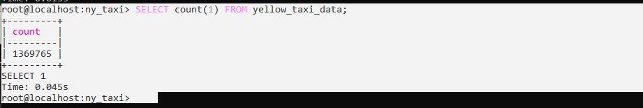
We can then run queries from there:

however we would be better to make use of a GUI tool which provides an improved visualization.

pgAdmin

pgAdmin is a web-based GUI tool used to interact with the Postgres database sessions, both locally and remote servers as well. It can be used to perform any sort of database administration required for a Postgres database. Although this is a GUI and can be installed, we don’t need to - we have Docker!

First we create a network to ensure that pgAdmin can talk to postgreSQL.

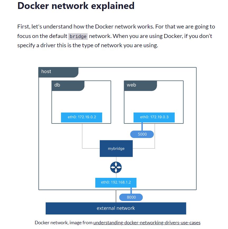
Where's that confounded bridge

The bridge network works as a private network internal to the host so containers on it can communicate. External access is granted by exposing ports to containers. Bridge networks are used when your applications run in standalone containers that need to communicate.

In the picture above db and web can communicate with each other on a user created bridge network called mybridge.

We can view the current networks running on our machine using:

docker network ls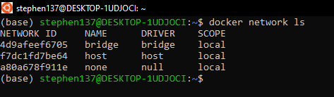

Docker inspect is a great way to retrieve low-level information on Docker objects. We can pick out any field from the returned JSON in a fairly straightforward manner.

So let’s use it to get the IP Address from the 2_docker_sql_pgadmin-1 container using :

       docker inspect -f '{{range .NetworkSettings.Networks}}{{.IPAddress}}{{end}}' <network ID>

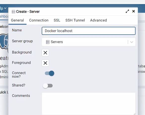
We can then just pull pgAdmin by running the folllowing from the command line :

docker run -it \
  -e PGADMIN_DEFAULT_EMAIL="admin@admin.com" \
  -e PGADMIN_DEFAULT_PASSWORD="root" \
  -p 8080:80 \
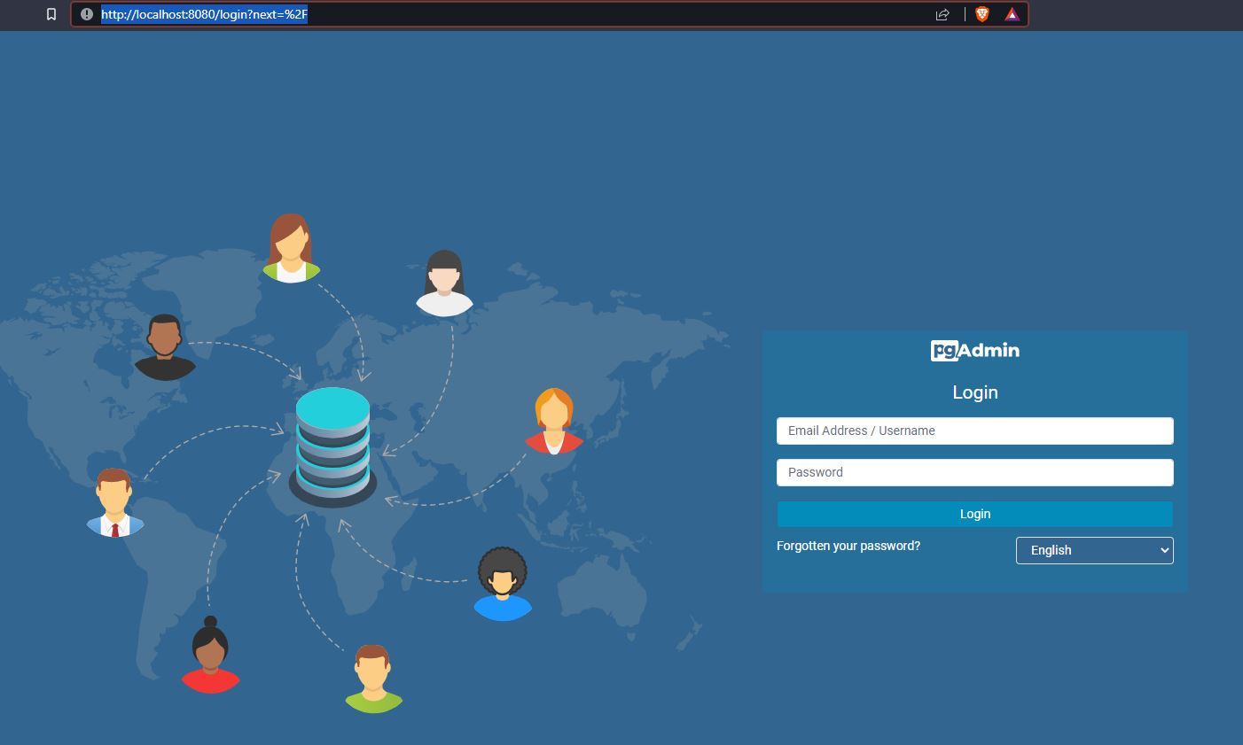
  dpage/pgadmin4

We then go to our browser and type:

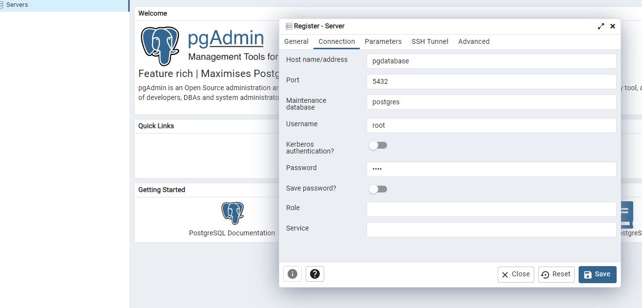
localhost8080

which takes us to the pgAdmin loginpage

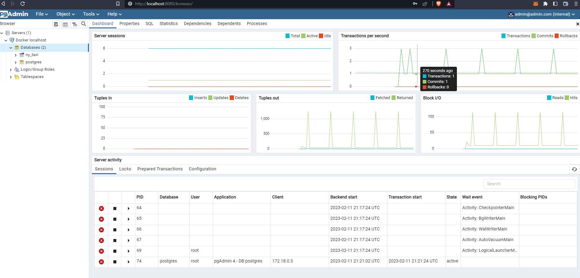
As we can see that has successfully loaded the data to postgres :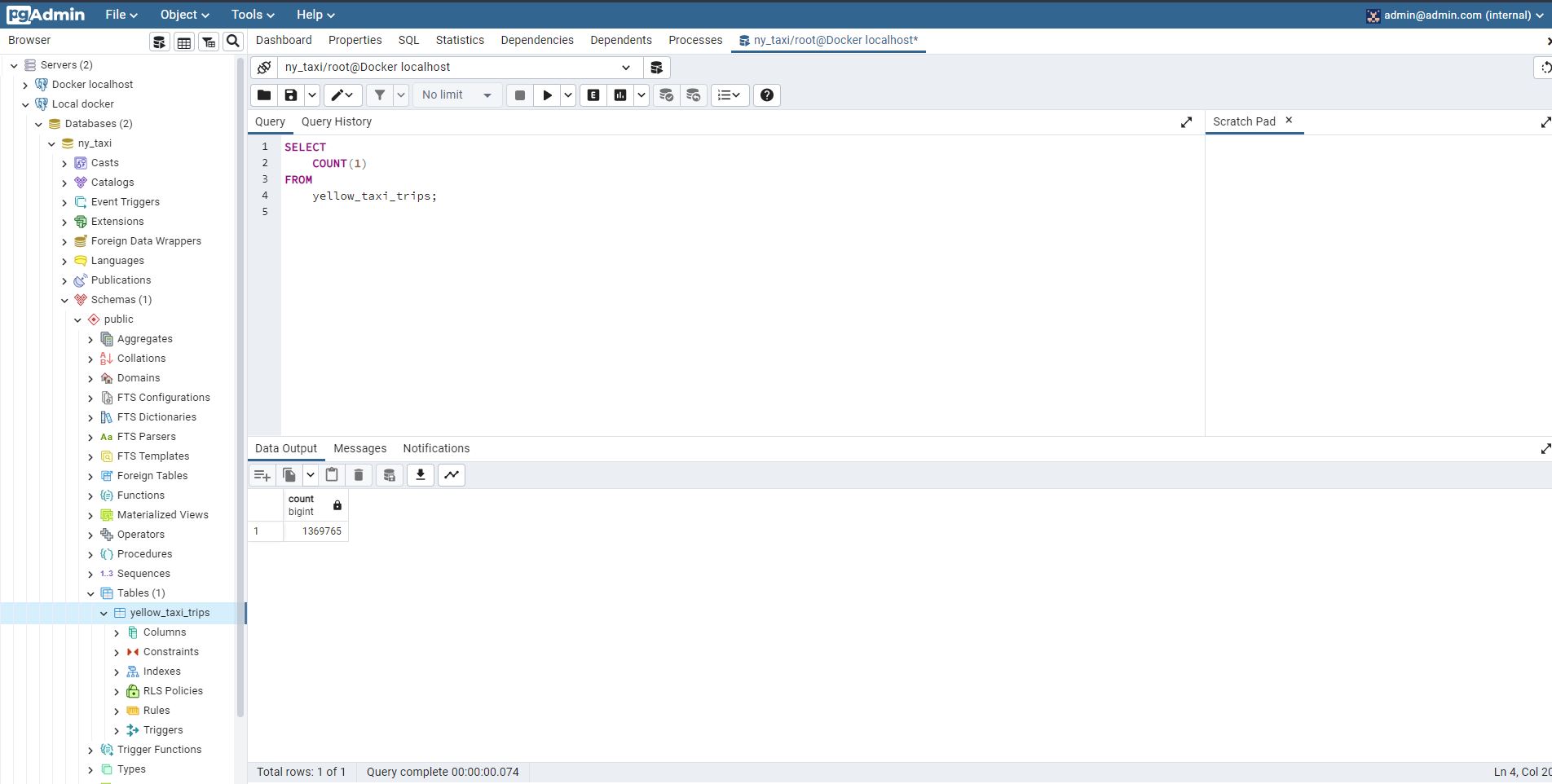

Docker-compose

Docker Container IP Address

By default, the container is assigned an IP address for every Docker network it connects to. And each network is created with a default subnet mask, using it as a pool later on to give away the IP addresses. Usually Docker uses the default 172.17. 0.0/16 subnet for container networking.

Now to better understand it, we will execute a real use case.

To illustrate this, we will use a postgreSQL and pgADmin environment, containing 2 Docker Containers, configured in the yaml file below:

services:
  pgdatabase:
    image: postgres:13
    environment:
      - POSTGRES_USER=root
      - POSTGRES_PASSWORD=root
      - POSTGRES_DB=ny_taxi
    volumes:
      - "./data/ny_taxi_postgres_data:/var/lib/postgresql/data:rw"
    ports:
      - "5432:5432"
  pgadmin:
    image: dpage/pgadmin4
    environment:
      - PGADMIN_DEFAULT_EMAIL=admin@admin.com
      - PGADMIN_DEFAULT_PASSWORD=root
    ports:
      - "8080:80"

Now let’s start up those containers using:

docker-compose up -d

and see the two containers by running the command:

docker ps --format "table {{.ID}}\t{{.Status}}\t{{.Names}}"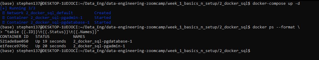

Next let’s check our Docker network using:

docker network ls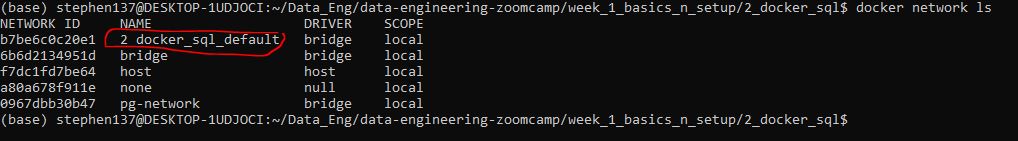

There’s a new network called 2_docker_sql_default. By default docker compose sets up a single network for your app. And your app’s network is given a name based on the “project name”, originated from the name of the directory it lives in. So since our directory is named 2_docker_sql, this explains the new network.

Next some examples on how to get the Docker IP Address.

How to Get A Docker Container IP Address

docker network inspect -f '{{range .IPAM.Config}}{{.Subnet}}{{end}}' b7be6c0c20e1

We don’t need to look up each Container’s IP individually:

docker network inspect -f '{{json .Containers}}' b7be6c0c20e1 | jq '.[] | .Name + ":" + .IPv4Address'

Note that we used jq help to parse the Containers map object which you may need to install.

So we can see the IP addresses of our containers :

pgdatabase-1 172.20.0.3 clear
pgadmin-1 172.20.0.2

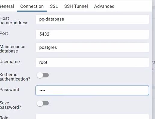
This could prove useful when mapping our database container to pgadmin.

1.2.4 Dockerizing our data ingestion file

We can introduce further automation by creating a python data ingest script which:

downloads the data
does some basic pre-processing
uploads the data in batches to postgresql

ingest_data.py

#!/usr/bin/env python
# coding: utf-8

import os
import argparse

from time import time

import pandas as pd
from sqlalchemy import create_engine


def main(params):
    user = params.user
    password = params.password
    host = params.host 
    port = params.port 
    db = params.db
    table_name = params.table_name
    url = params.url

    # the backup files are gzipped, and it's important to keep the correct extension
    # for pandas to be able to open the file
    if url.endswith('.csv.gz'):
        csv_name = 'output.csv.gz'
    else:
        csv_name = 'output.csv'

os.system(f"wget {url} -O {csv_name}")

engine = create_engine(f'postgresql://{user}:{password}@{host}:{port}/{db}')

df_iter = pd.read_csv(csv_name, iterator=True, chunksize=100000)

df = next(df_iter)

df.tpep_pickup_datetime = pd.to_datetime(df.tpep_pickup_datetime)
df.tpep_dropoff_datetime = pd.to_datetime(df.tpep_dropoff_datetime)

df.head(n=0).to_sql(name=table_name, con=engine, if_exists='replace')

df.to_sql(name=table_name, con=engine, if_exists='append')


while True: 

    try:
        t_start = time()
        
        df = next(df_iter)

        df.tpep_pickup_datetime = pd.to_datetime(df.tpep_pickup_datetime)
        df.tpep_dropoff_datetime = pd.to_datetime(df.tpep_dropoff_datetime)

        df.to_sql(name=table_name, con=engine, if_exists='append')

        t_end = time()

        print('inserted another chunk, took %.3f second' % (t_end - t_start))

    except StopIteration:
        print("Finished ingesting data into the postgres database")
        break

if __name__ == '__main__':
    parser = argparse.ArgumentParser(description='Ingest CSV data to Postgres')

    parser.add_argument('--user', required=True, help='user name for postgres')
    parser.add_argument('--password', required=True, help='password for postgres')
    parser.add_argument('--host', required=True, help='host for postgres')
    parser.add_argument('--port', required=True, help='port for postgres')
    parser.add_argument('--db', required=True, help='database name for postgres')
    parser.add_argument('--table_name', required=True, help='name of the table where we will write the results to')
    parser.add_argument('--url', required=True, help='url of the csv file')

    args = parser.parse_args()

    main(args)

This command line prompt runs the python data ingest file :

Create our network :

docker network create pg-network

Run Postgres (change the path) :

  docker run -it \
  -e POSTGRES_USER="root" \
  -e POSTGRES_PASSWORD="root" \
  -e POSTGRES_DB="ny_taxi" \
  -v $(pwd)/ny_taxi_postgres_data:/var/lib/postgresql/data \
  -p 5432:5432 \
  --network=pg-network \
  --name pg-database \
  postgres:13

Run pgAdmin :

docker run -it \
  -e PGADMIN_DEFAULT_EMAIL="admin@admin.com" \
  -e PGADMIN_DEFAULT_PASSWORD="root" \
  -p 8080:80 \
  dpage/pgadmin4

URL="https://github.com/DataTalksClub/nyc-tlc-data/releases/download/yellow/yellow_tripdata_2021-01.csv.gz"

python ingest_data.py \
  --user=root \
  --password=root \
  --host=localhost \
  --port=5432 \
  --db=ny_taxi \
  --table_name=yellow_taxi_trips \
  --url=${URL}

Using docker

Create the following Dockerfile :

FROM python:3.9.1

RUN apt-get install wget    
RUN pip install pandas sqlalchemy psycopg2  

WORKDIR /app
COPY ingest_data.py ingest_data.py

ENTRYPOINT [ "python", "ingest_data.py" ]

Then run the following command line prompts :

docker build -t taxi_ingest:v001 .

Running this throws up the following error:

Docker - failed to solve with frontend dockerfile.v0: failed to read dockerfile: error from sender: open ny_taxi_postgres_data: permission denied.

This happens on Ubuntu/Linux systems when trying to run the command to build the Docker container again. A folder is created to host the Docker files. When the build command is executed again to rebuild the pipeline or create a new one the error is raised as there are no permissions on this new folder. Grant permissions by running this command :

sudo chmod -R 755 ny_taxi_postgres_data

Now we can run the ingest_data.py script from the command line :

URL="https://github.com/DataTalksClub/nyc-tlc-data/releases/download/yellow/yellow_tripdata_2021-01.csv.gz"

docker run -it \
  --network=pg-network \
  taxi_ingest:v001 \
    --user=root \
    --password=root \
    --host=pg-database \
    --port=5432 \
    --db=ny_taxi \
    --table_name=yellow_taxi_trips \

    --url=${URL}

To get all the files on a localhost directory we can run the following command:

python -m http.server

To get the IP address of your computer you can run :

ifconfig

1.2.5 Docker Compose

In the previous section we:

ran postgres
ran pgAdmin

in one network using two docker commands.

This works fine but there is a lot of configuration required. We can streamline the process by pooling everything together in one yaml file where we can configure multiple CONTAINERS. We can then run from the command line using docker-compose :

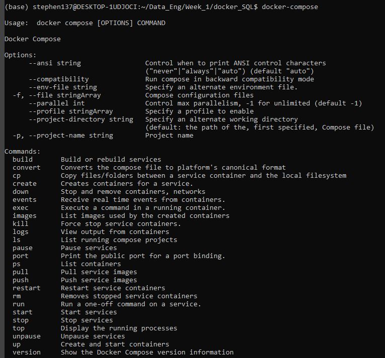
Let’s try docker-compose from the command line :

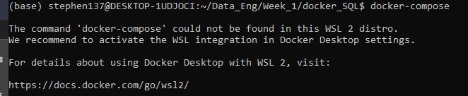
Docker Compose comes as part of Windows Docker Desktop, but if like me, you are running things in Linux from the Ubuntu command line, then you need to activate the WSL integration:

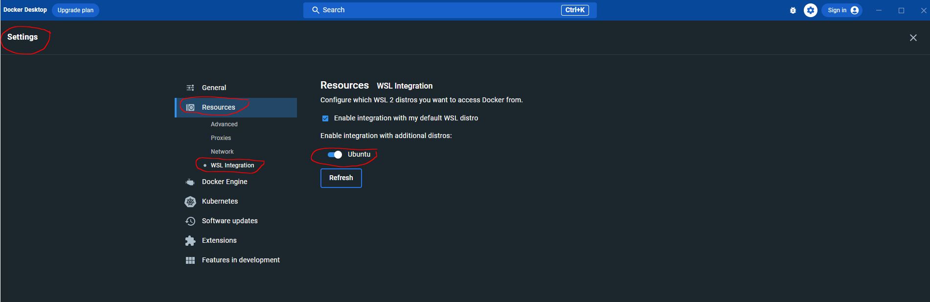
Running docker-compose now works:

We can now create our yaml file named docker-compose.yaml :

services:
  pgdatabase:
    image: postgres:13
    environment:
      - POSTGRES_USER=root
      - POSTGRES_PASSWORD=root
      - POSTGRES_DB=ny_taxi
    volumes:
      - "./ny_taxi_postgres_data:/var/lib/postgres/data:rw"
    ports:
      - "5432:5432"
  pgadmin:
    image: dpage/pgadmin4
    environment:
      - PGADMIN_DEFAULT_EMAIL=admin@admin.com
      - PGADMIN_DEFAULT_PASSWORD=root
    ports:
      - "8080:80"

Ensure all existing containers, volumes and images are cleared and run using :

docker-compose up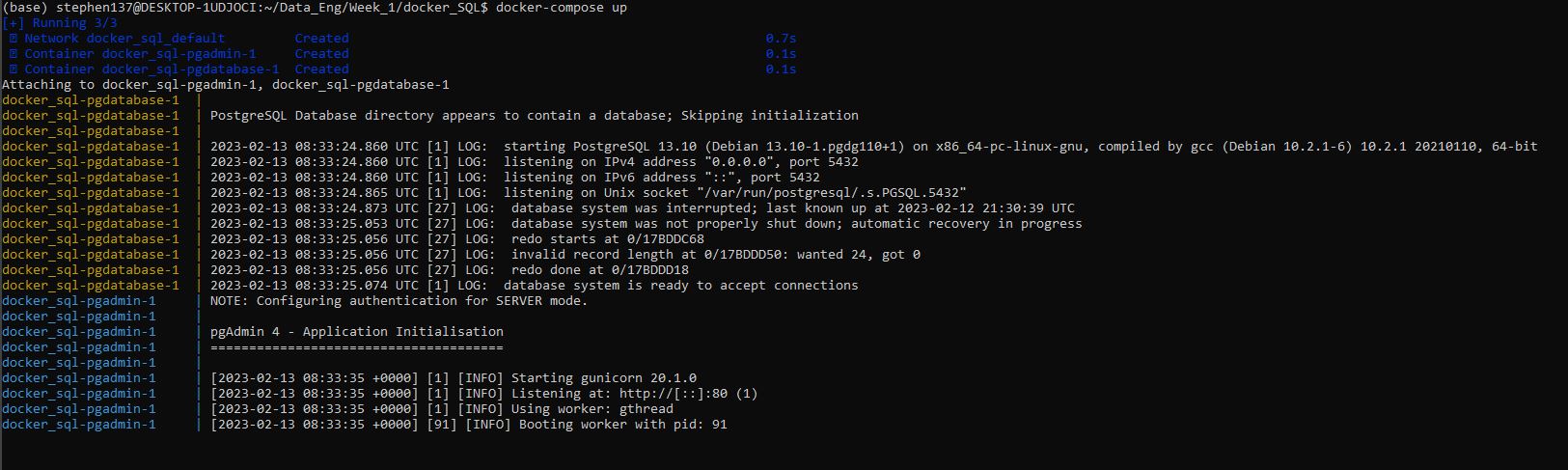

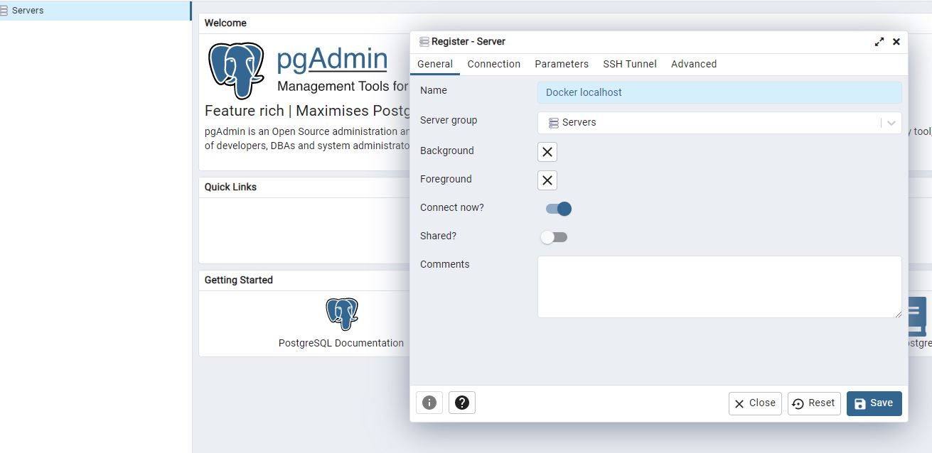
Then we go to localhost 8080 and use the pgAdmin login details configured in the yaml file. Unfortunately the yaml file is not configured to ensure persistent state for pgAdmin, so we have to register a server again.

We can close the terminal using CTRL + C but then we should also run docker-compose down.

A better way is to run with docker-compose up -d runs in detached mode which then allows us to bypass CTRL + C and go straight to docker-compose down.

1.2.6 - SQL Refresher

df_zones = pd.read_csv('Data/taxi_zone_lookup.csv')

Take a look at the first 5 rows :

df_zones.head(140)

	LocationID	Borough	Zone	service_zone
0	1	EWR	Newark Airport	EWR
1	2	Queens	Jamaica Bay	Boro Zone
2	3	Bronx	Allerton/Pelham Gardens	Boro Zone
3	4	Manhattan	Alphabet City	Yellow Zone
4	5	Staten Island	Arden Heights	Boro Zone
...	...	...	...	...
135	136	Bronx	Kingsbridge Heights	Boro Zone
136	137	Manhattan	Kips Bay	Yellow Zone
137	138	Queens	LaGuardia Airport	Airports
138	139	Queens	Laurelton	Boro Zone
139	140	Manhattan	Lenox Hill East	Yellow Zone

140 rows × 4 columns

Upload to postgres :

from sqlalchemy import create_engine

engine = create_engine('postgresql://root:root@localhost:5432/ny_taxi')

df_zones.to_sql(name='zones', con=engine, if_exists='replace')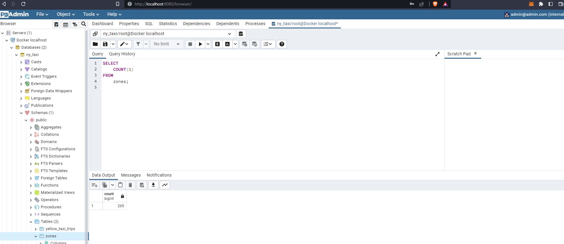

Let’s now carry out some SQL queries on our tables:

yellow_taxi_trips
zones

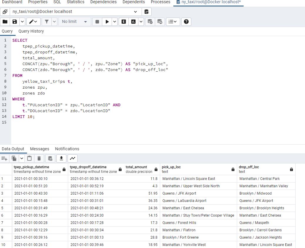
Joining tables in SQL

It will be useful to join these tables. There are different ways to do this. First let’s look at query which returns specified columns which combine certain information common to both tables - in this case LocationID :

Another way to construct the query is to explicitly use the JOIN command:

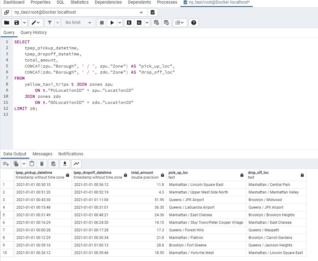
Both queries are equivalent.

Say, we wanted to check for pick up or drop off locations which are in one table but not the other:

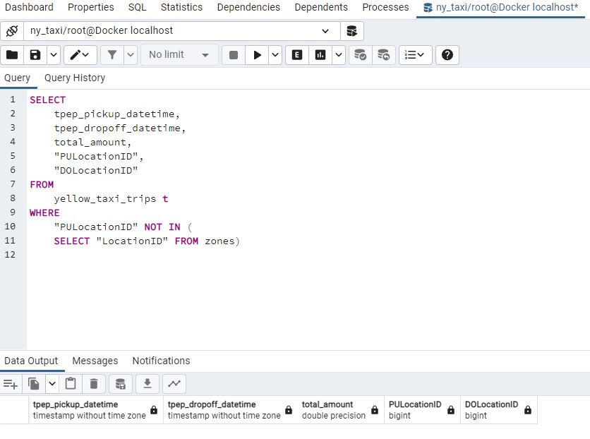
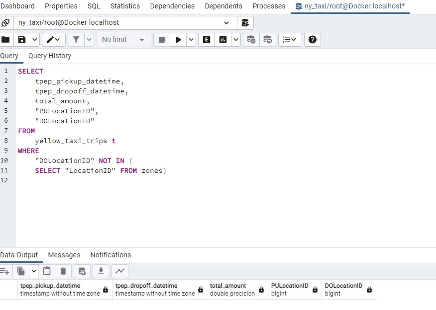
Both queries return no records so that means that all the records have pick up and drop off locations and all the IDs in the zones table are present in the taxis table. In some cases there might not be fully matching records. In this case we can use other join methods :

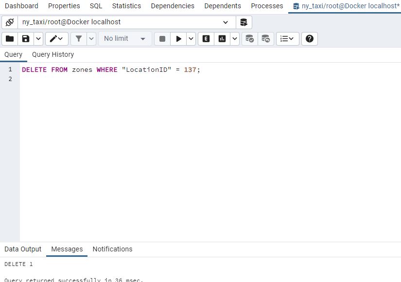
For illustration purposes let’s remove a LocationID record from our zones table:

And now when we query records that don’t match :

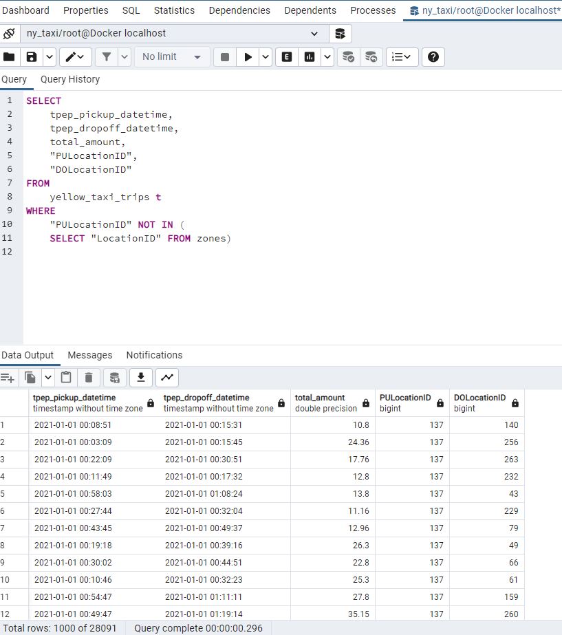
We can use LEFT JOIN which will still return a record even where LocationID is not available :

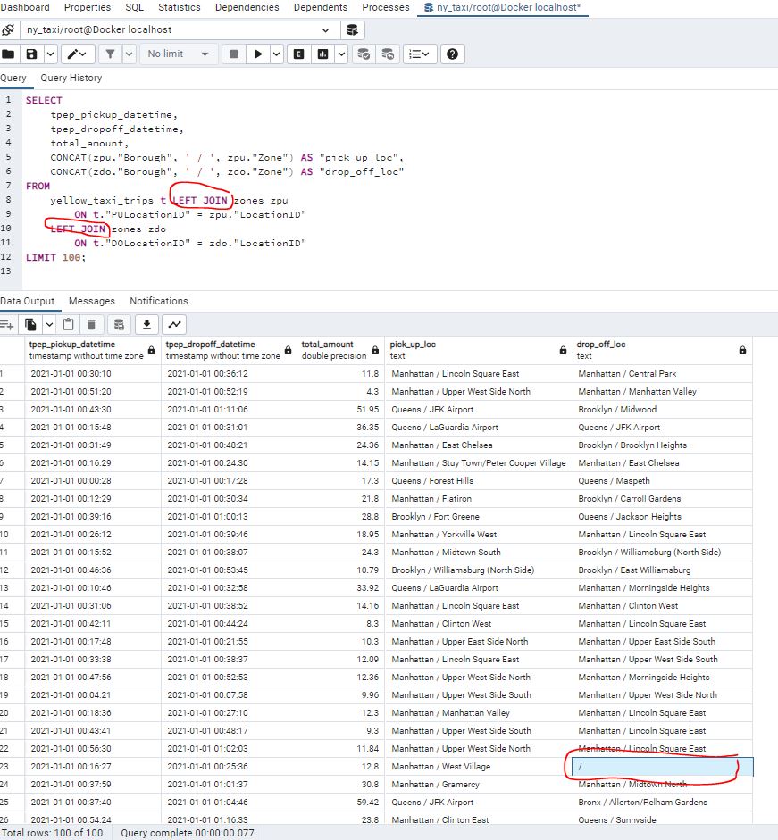
There are also RIGHT JOIN and OUTER JOIN statements but these will be covered further in Week 4 .

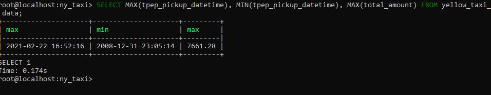
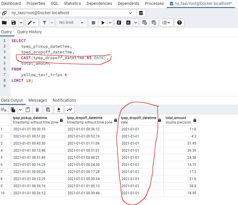
Working with dates

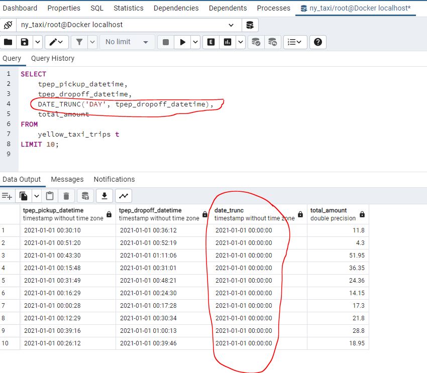
Aggregating in SQL

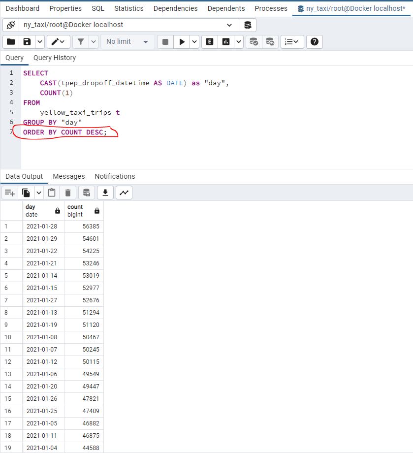
Say we wanted to find how many records there were for each day. We can build on our date parsing above and use a GROUP BY and ORDER BY query :

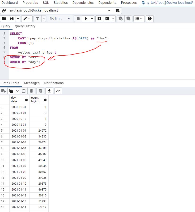
If we wanted to see the day with the largest number of records we coud order by count:

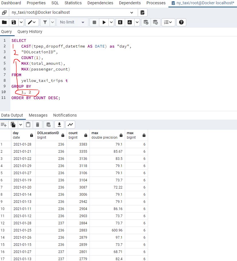
We can use a variety of aggregation methods. Note that we can use numbers to reference the ordering of GROUP BY :

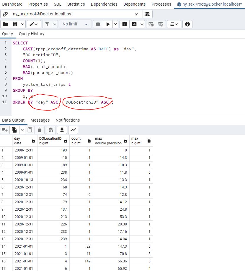
We can also include multiple conditions in our ORDER BY clause :

1.3.1 Introduction to Terraform Concepts & GCP Pre-Requisites

Terraform is an open-source infrastructure-as-code software tool created by HashiCorp. Users define and provide data center infrastructure using a declarative configuration language known as HashiCorp Configuration Language, or optionally JSON.

Build, change, and destroy Google Cloud Platform (GCP) infrastructure using Terraform. Step-by-step, command-line tutorials will walk you through the Terraform basics for the first time.

https://learn.hashicorp.com/collections/terraform/gcp-get-started

Terraform can be installed using the following command line prompts in Ubuntu:

wget -O- https://apt.releases.hashicorp.com/gpg | gpg --dearmor | sudo tee /usr/share/keyrings/hashicorp-archive-keyring.gpg \
echo "deb [signed-by=/usr/share/keyrings/hashicorp-archive-keyring.gpg] https://apt.releases.hashicorp.com $(lsb_release -cs) main" | sudo tee\ /etc/apt/sources.list.d/hashicorp.list
sudo apt update && sudo apt install terraform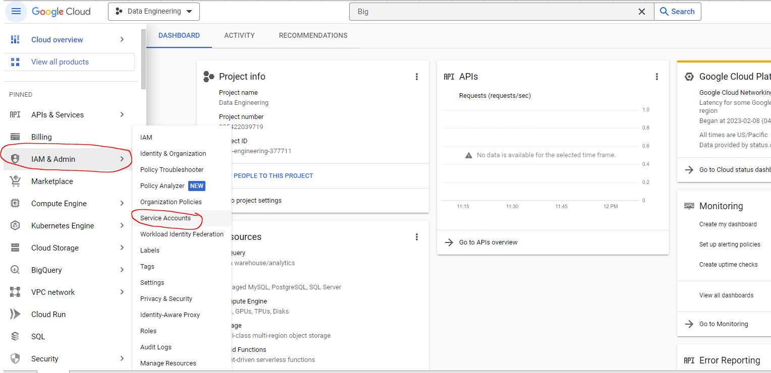

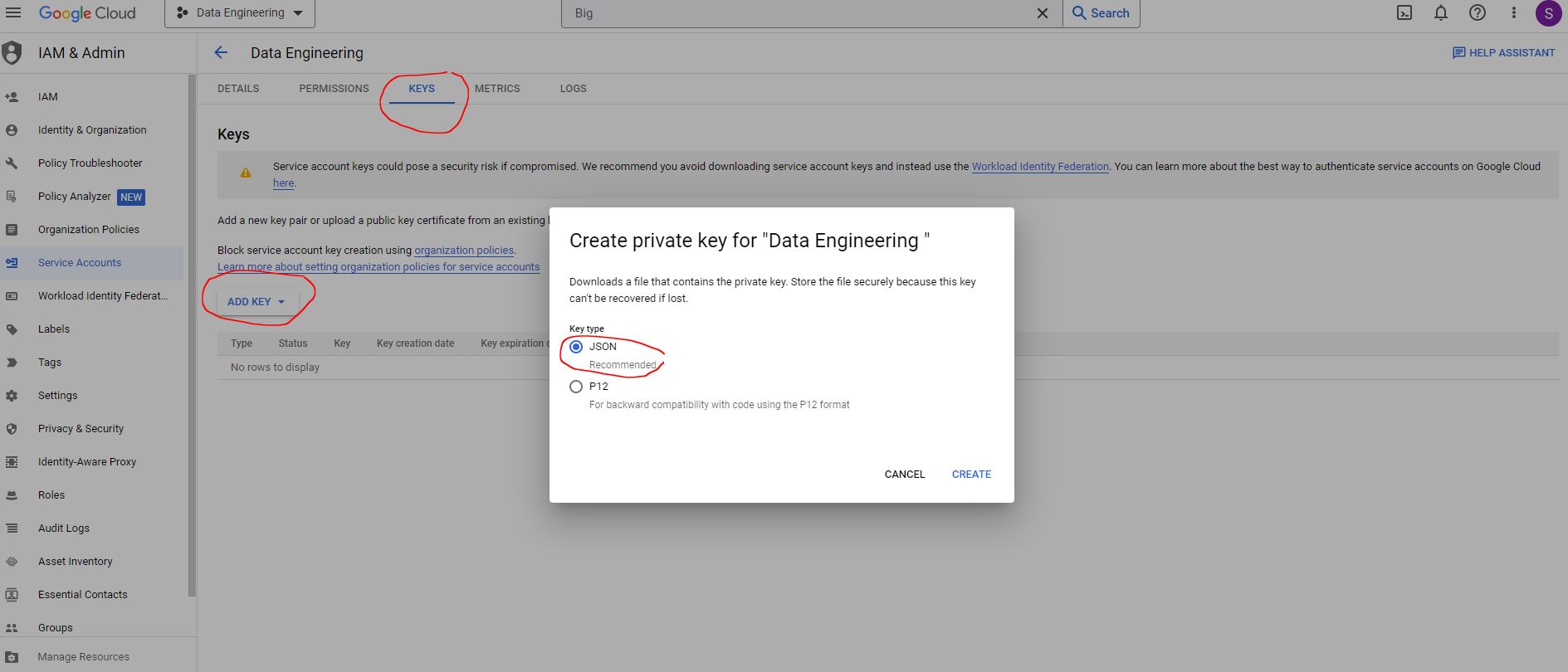
This will download a key in json format

Cloud SDK

Cloud SDK provides language-specific Cloud Client Libraries supporting each language’s natural conventions and styles. This makes it easier for you to interact with Google Cloud APIs in your language of choice. Client libraries also handle authentication, reduce the amount of necessary boilerplate code, and provide helper functions for pagination of large datasets and asynchronous handling of long-running operations.

To check if we have it installed we can run the following prompt at the command line :

gcloud -v

I did not have it so need to install:

https://cloud.google.com/sdk/docs/install-sdk#deb

Installation of gcloud CLI

Add the gcloud CLI distribution URI as a package source. If your distribution supports the signed-by option, run the following command:

echo “deb [signed-by=/usr/share/keyrings/cloud.google.gpg] https://packages.cloud.google.com/apt cloud-sdk main” | sudo tee -a /etc/apt/sources.list.d/google-cloud-sdk.list
Import the Google Cloud public key. If your distribution’s apt-key command supports the –keyring argument, run the following command:

curl https://packages.cloud.google.com/apt/doc/apt-key.gpg | sudo apt-key –keyring /usr/share/keyrings/cloud.google.gpg add -
Update and install the gcloud CLI:

sudo apt-get update && sudo apt-get install google-cloud-cli
(Optional) Install any of the additional components.
Run gcloud init to get started:

gcloud init

Say yes to the above, and then in your browser, log in to your Google user account when prompted and click Allow to grant permission to access Google Cloud resources. Copy the verification code to the awaiting command line prompt
At the command prompt, select a Google Cloud project from the list of projects where you have Owner, Editor or Viewer permissions:
If you have the Compute Engine API enabled, gcloud init allows you to choose a default Compute Engine zone:

(Optional) To improve the screen reader experience, enable the accessibility/screen_reader property:

gcloud config set accessibility/screen_reader true

Now we need to export our key credentials from the json file at the command line:

export GOOGLE_APPLICATION_CREDENTIALS=$(pwd)/<json_file_name>.json

Finally, refresh token/session, and verify authentication:

gcloud auth application-default login

Then need to login from the browser to Google account once again and Allow and then copy verification code to terminal:

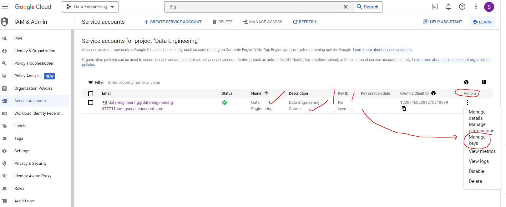
We are now going to set up the following infrastructures within Google Cloud Platform (GCP):

- Google Cloud Storage (GCS): (a bucket in GCP environment where you can store files) Data Lake - raw data in organised fashion 
- Big Query: Data Warehouse

We need to grant two additional service permissions:

Storage Admin (the bucket itself) and Storage Object Admin (the objects within the bucket)
BigQuery Admin

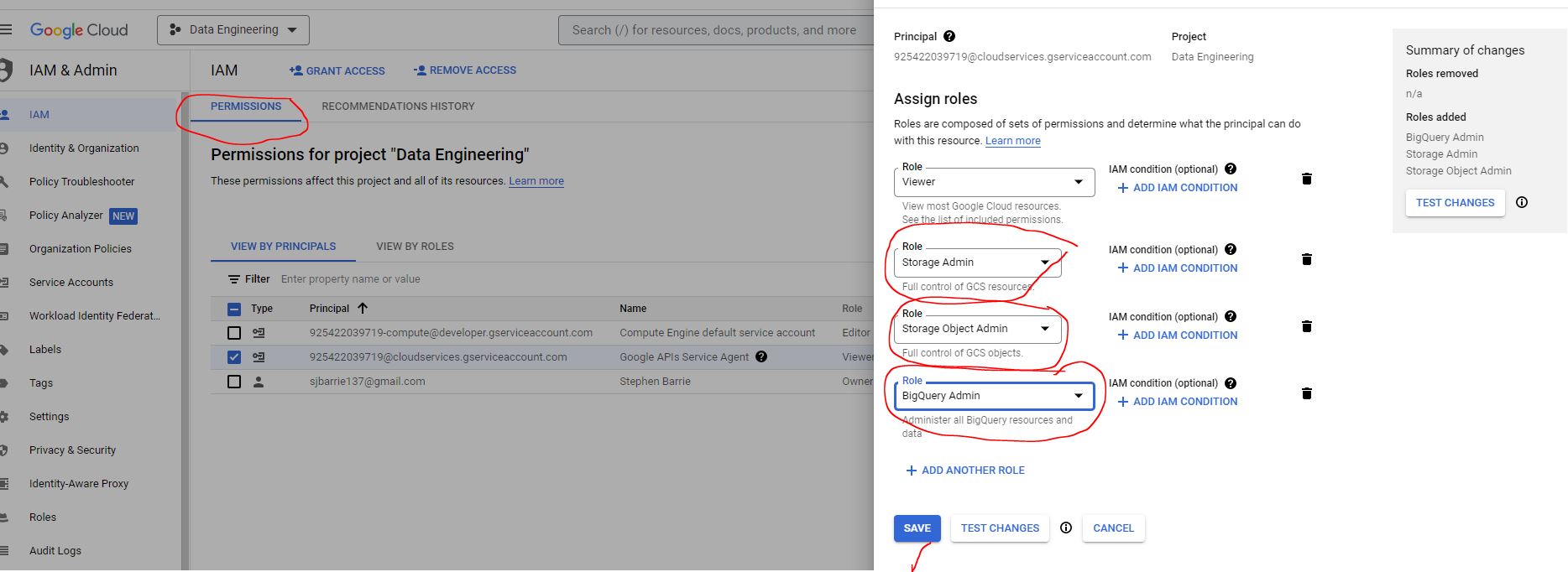
In production there would be custom created access parameters, restricting access by certain people to certain files.

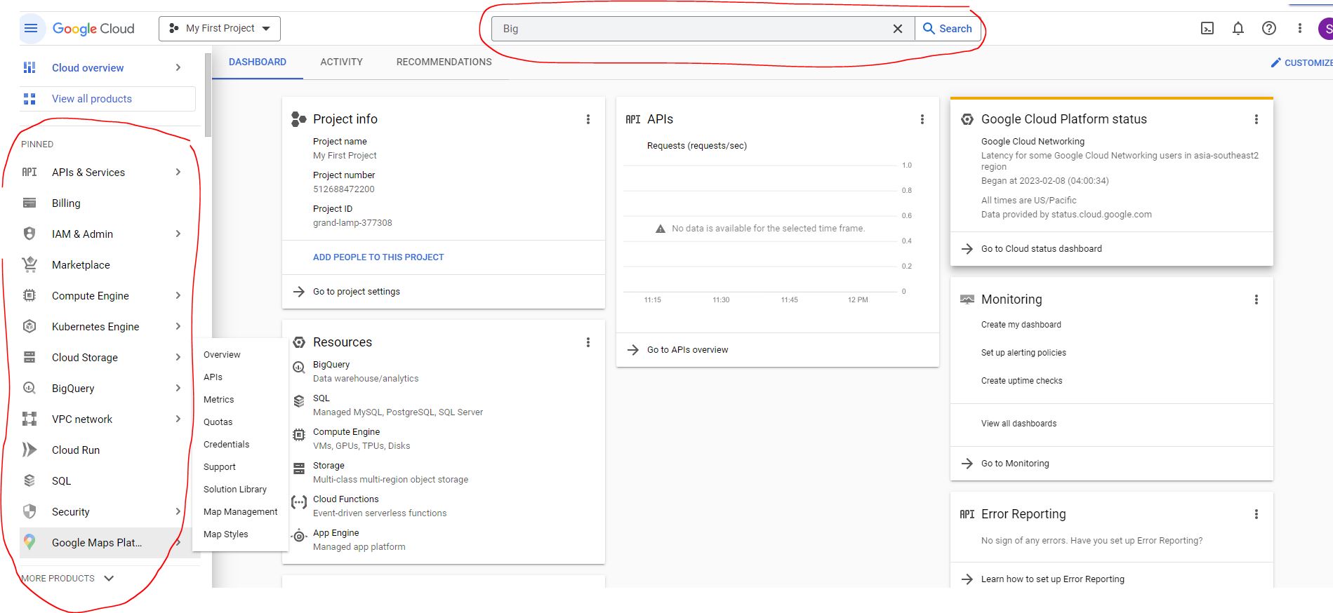
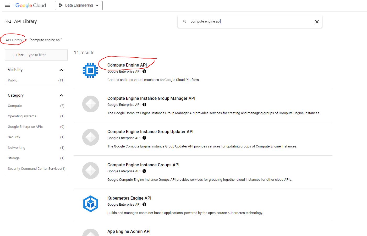
We still require to enable the APIs:

https://console.cloud.google.com/apis/library/iam.googleapis.com

https://console.cloud.google.com/apis/library/iamcredentials.googleapis.com

1.3.2 Creating GCP Infrastructure with Terraform

Now that we have everything set up within GCP let’s get started with the Terraform config. We need two files :

main.tf (which references the variables.tf file)
variables.tf

main.tf

terraform {
  required_version = ">= 1.0"
  backend "local" {}  # Can change from "local" to "gcs" (for google) or "s3" (for aws), if you would like to preserve your tf-state online
  required_providers {
    google = {
      source  = "hashicorp/google"
    }
  }
}

provider "google" {
  project = var.project
  region = var.region
  // credentials = file(var.credentials)  # Use this if you do not want to set env-var GOOGLE_APPLICATION_CREDENTIALS
}

# Data Lake Bucket
# Ref: https://registry.terraform.io/providers/hashicorp/google/latest/docs/resources/storage_bucket
resource "google_storage_bucket" "data-lake-bucket" {
  name          = "${local.data_lake_bucket}_${var.project}" # Concatenating DL bucket & Project name for unique naming
  location      = var.region

  # Optional, but recommended settings:
  storage_class = var.storage_class
  uniform_bucket_level_access = true

  versioning {
    enabled     = true
  }

      lifecycle_rule {
    action {
      type = "Delete"
    }
    condition {
      age = 30  // days
    }
  }

  force_destroy = true
}

# DWH
# Ref: https://registry.terraform.io/providers/hashicorp/google/latest/docs/resources/bigquery_dataset
resource "google_bigquery_dataset" "dataset" {
  dataset_id = var.BQ_DATASET
  project    = var.project
  location   = var.region

variables.tf

locals {
  data_lake_bucket = "dtc_data_lake"
}

variable "project" {
  description = "data-engineering-377711"
}

variable "region" {
  description = "Region for GCP resources. Choose as per your location: https://cloud.google.com/about/locations"
  default = "europe-west6"
  type = string
}

variable "storage_class" {
  description = "Storage class type for your bucket. Check official docs for more info."
  default = "STANDARD"
}

variable "BQ_DATASET" {
  description = "BigQuery Dataset that raw data (from GCS) will be written to"
  type = string
  default = "trips_data_all"
}

Once we have configured the above Terraform files, there are only a few execution commands which makes it very convenient to work with.

terraform init: - Initializes & configures the backend, installs plugins/providers, & checks out an existing configuration from a version control

terraform plan: - Matches/previews local changes against a remote state, and proposes an Execution Plan.

terraform apply: - Asks for approval to the proposed plan, and applies changes to cloud

!!!terraform destroy!!!: - Removes your stack from the Cloud

Let’s initialize state file (.tfstate) from the command line using

terraform init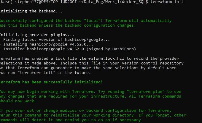

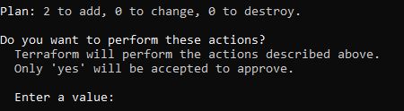
Next, propose an execution plan using

terraform plan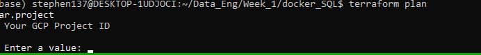

We need to enter our GCP Project ID at the command prompt to progress.

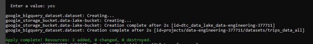
Now let’s ask for approval to the proposed plan, and apply the changes to cloud using

terraform apply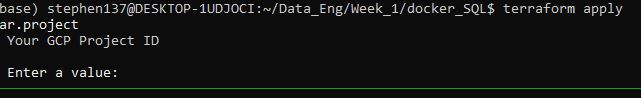

Once again, we need to enter our GCP Project ID at the command prompt to progress:

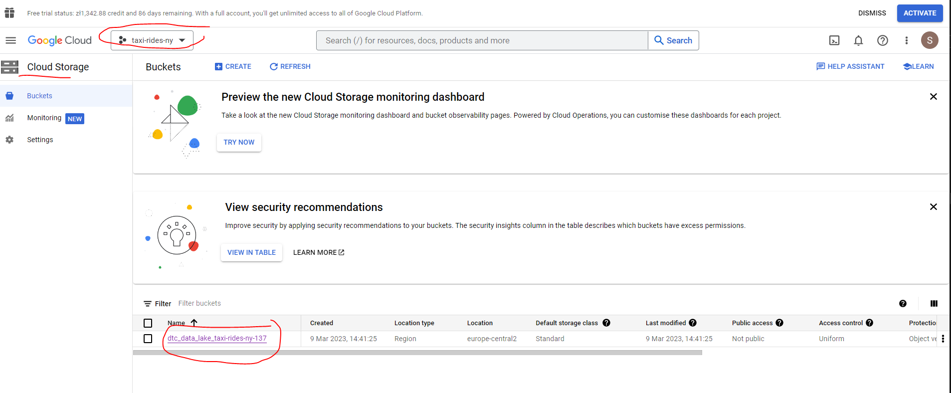
We’re all set! Let’s return to our GCP account and confirm that we do now have a data lake bucket :

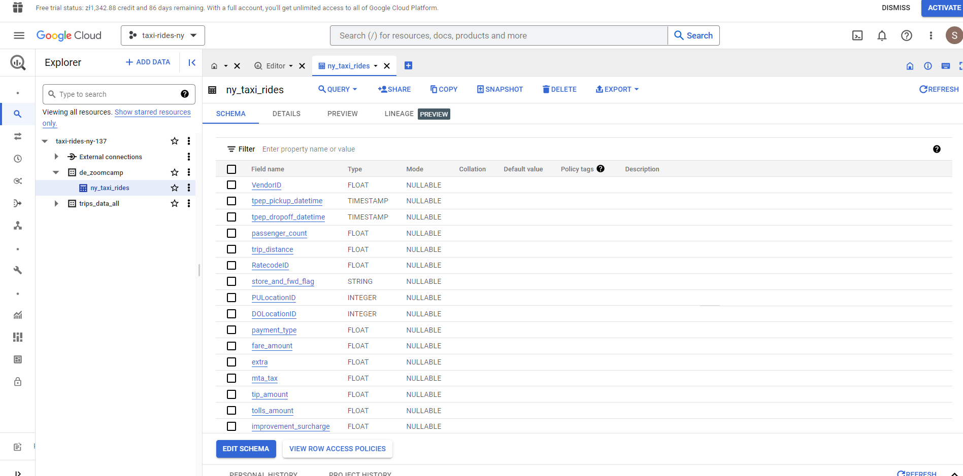
And also check that we have our Big Query :

Key Takeaways

The intro video to the course did stress that the set up would take more than a week! I started the set up on my own machine using Ubuntu on Windows 10 but ran into some dependency issues. I then went through the process for setting up a Virtual Machine on Google Cloud, but wasn’t completely comfortable working within that environment so in the end I went full circle and managed to resolve the previous issues I was having. Onwards and upwards! Looking forward to “Week 2” Workflow Orchestration.