# install fastkaggle if not available
try: import fastkaggle
except ModuleNotFoundError:
    !pip install -Uq fastkaggle

from fastkaggle import *This is my follow up to the second part of Lesson 6: Practical Deep Learning for Coders 2022 in which Jeremy walks us through his approach to obtaining the top score on the Paddy Doctor: Paddy Disease Classification Kaggle competition.
Problem Statement - identify the type of disease present in paddy leaf images
Rice (Oryza sativa) is one of the staple foods worldwide. Paddy, the raw grain before removal of husk, is cultivated in tropical climates, mainly in Asian countries. Paddy cultivation requires consistent supervision because several diseases and pests might affect the paddy crops, leading to up to 70% yield loss. Expert supervision is usually necessary to mitigate these diseases and prevent crop loss. With the limited availability of crop protection experts, manual disease diagnosis is tedious and expensive. Thus, it is increasingly important to automate the disease identification process by leveraging computer vision-based techniques that achieved promising results in various domains.
Objective
The main objective of the competition is to develop a machine or deep learning-based model to classify the given paddy leaf images accurately. A training dataset of 10,407 (75%) labeled images across ten classes (nine disease categories and normal leaf) is provided. Moreover, also provided is additional metadata for each image, such as the paddy variety and age. Our task is to classify each paddy image in the given test dataset of 3,469 (25%) images into one of the nine disease categories or a normal leaf.
Approach
In Iterate Like a Grandmaster Jeremy Howard explained that when working on a Kaggle project:
…the focus generally should be two things:
- Creating an effective validation set
- Iterating rapidly to find changes which improve results on the validation set
Here we’re going to go further, showing the process he used to tackle the Paddy Doctor competition, leading to four submissions in a row which all were (at the time of submission) in 1st place, each one more accurate than the last. You might be surprised to discover that the process of doing this was nearly entirely mechanistic and didn’t involve any consideration of the actual data or evaluation details at all.
This notebook shows every step of the process. At the start of this notebook we’ll make a basic submission; by the end we’ll see how he got to the top of the table!:

As a special extra, also included is a selection of “walkthru” videos that were prepared for the new fast.ai course, and cover this competition:
Getting set up
First, we’ll get the data. There’s a new library called fastkaggle which has a few handy features, including getting the data for a competition correctly regardless of whether we’re running on Kaggle or elsewhere. Note we’ll need to first accept the competition rules and join the competition, and we’ll need our kaggle API key file kaggle.json downloaded if you’re running this somewhere other than on Kaggle. setup_comp is the function we use in fastkaggle to grab the data, and install or upgrade our needed python modules when we’re running on Kaggle:
::: {.cell _kg_hide-output=‘true’ execution_count=10}
comp = 'paddy-disease-classification'

path = setup_comp(comp, install='fastai "timm>=0.6.2.dev0"')
:::
pathPath('paddy-disease-classification')Now we can import the stuff we’ll need from fastai, set a seed (for reproducibility – just for the purposes of making this notebook easier to write; It’s not recommended to do that in your own analysis however) and check what’s in the data:
from fastai.vision.all import *
set_seed(42)

path.ls()
(#4) [Path('paddy-disease-classification/sample_submission.csv'),Path('paddy-disease-classification/test_images'),Path('paddy-disease-classification/train_images'),Path('paddy-disease-classification/train.csv')]Looking at the data
The images are in train_images, so let’s grab a list of all of them:
trn_path = path/'train_images'
files = get_image_files(trn_path)
…and take a look at one:
img = PILImage.create(files[0])
print(img.size)
img.to_thumb(128)
(480, 640)
Looks like the images might be 480x640 – let’s check all their sizes. This is faster if we do it in parallel, so we’ll use fastcore’s parallel for this:
Watch out! In the imaging world images are represented by (columns, rows) however in the array/tensor world images are represented as (rows, columns). Pytorch would say size is (640, 480)!!
from fastcore.parallel import *

# create function to create a PILLOW image and get its size
# speed up process using parallel
def f(o): return PILImage.create(o).size
sizes = parallel(f, files, n_workers=8)
pd.Series(sizes).value_counts()
(480, 640) 10403
(640, 480) 4
dtype: int64They’re nearly all the same size, except for a few. Because of those few, however, we’ll need to make sure we always resize each image to common dimensions first, otherwise fastai won’t be able to create batches. For now, we’ll just squish them to 480x480 images, and then once they’re in batches we do a random resized crop down to a smaller size, along with the other default fastai augmentations provided by aug_transforms. We’ll start out with small resized images, since we want to be able to iterate quickly:
# create our dataloader
dls = ImageDataLoaders.from_folder(trn_path, valid_pct=0.2, seed=42,
    item_tfms=Resize(480, method='squish'), # resize to a 480 x 480 square using squish - change aspect ratio
    batch_tfms=aug_transforms(size=128, min_scale=0.75))

#  show_batch allows us to see or hear our data
dls.show_batch(max_n=6)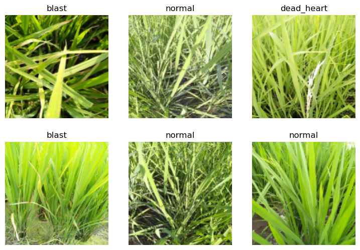
Our first model
Let’s create a model. To pick an architecture, we should look at the options in The best vision models for fine-tuning. resnet26d is the fastest resolution-independent model which gets into the top-15 lists there.
learn = vision_learner(dls, 'resnet26d', metrics=error_rate, path='.').to_fp16()Downloading: "https://github.com/rwightman/pytorch-image-models/releases/download/v0.1-weights/resnet26d-69e92c46.pth" to /home/stephen137/.cache/torch/hub/checkpoints/resnet26d-69e92c46.pthLet’s see what the learning rate finder shows:
# puts through one mini-batch at a time, starting at a very low learning rate
# gradually increase learning rate, see improvement, then once lr gets bigger worsens
learn.lr_find(suggest_funcs=(valley, slide))
/home/stephen137/mambaforge/lib/python3.10/site-packages/torch/amp/autocast_mode.py:198: UserWarning: User provided device_type of 'cuda', but CUDA is not available. Disabling
warnings.warn('User provided device_type of \'cuda\', but CUDA is not available. Disabling')
/home/stephen137/mambaforge/lib/python3.10/site-packages/torch/cuda/amp/grad_scaler.py:115: UserWarning: torch.cuda.amp.GradScaler is enabled, but CUDA is not available. Disabling.
warnings.warn("torch.cuda.amp.GradScaler is enabled, but CUDA is not available. Disabling.")SuggestedLRs(valley=0.0014454397605732083, slide=0.0030199517495930195)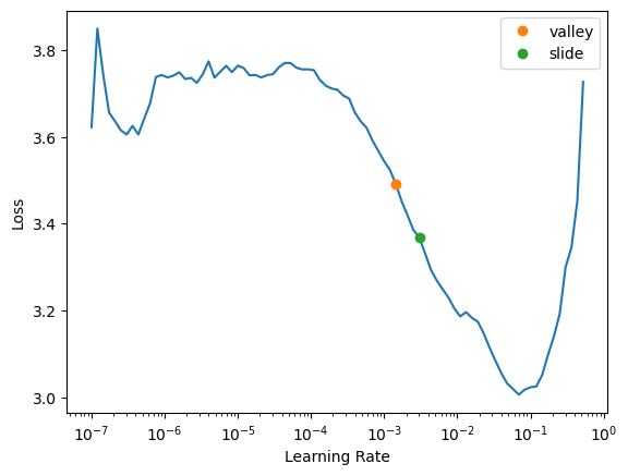
lr_find generally recommends rather conservative learning rates, to ensure that your model will train successfully. I generally like to push it a bit higher if I can. Let’s train a few epochs and see how it looks:
# let's fine tune for 3 epochs with a selected learning rate of 0.01 (10 ^ -2)
learn.fine_tune(3, 0.01)| epoch | train_loss | valid_loss | error_rate | time |
|---|---|---|---|---|
| 0 | 1.774996 | 1.171467 | 0.378664 | 03:57 |
| epoch | train_loss | valid_loss | error_rate | time |
|---|---|---|---|---|
| 0 | 1.074707 | 0.791964 | 0.265257 | 04:52 |
| 1 | 0.786653 | 0.482838 | 0.144161 | 04:59 |
| 2 | 0.534015 | 0.414971 | 0.129265 | 05:00 |
We’re now ready to build our first submission!!! Let’s take a look at the sample Kaggle provided to see what it needs to look like:
Submitting to Kaggle
# lets's have a look at the sample Kaggle submisison file
ss = pd.read_csv(path/'sample_submission.csv')
ss| image_id | label | |
|---|---|---|
| 0 | 200001.jpg | NaN |
| 1 | 200002.jpg | NaN |
| 2 | 200003.jpg | NaN |
| 3 | 200004.jpg | NaN |
| 4 | 200005.jpg | NaN |
| ... | ... | ... |
| 3464 | 203465.jpg | NaN |
| 3465 | 203466.jpg | NaN |
| 3466 | 203467.jpg | NaN |
| 3467 | 203468.jpg | NaN |
| 3468 | 203469.jpg | NaN |
3469 rows × 2 columns
OK so we need a CSV containing all the test images, in alphabetical order, and the predicted label for each one. We can create the needed test set using fastai like so:
# create our test set
tst_files = get_image_files(path/'test_images').sorted()

# create a dataloader pointing at the test set - use dls.test_dl
# key difference from normal dataloader is that it does not have any labels
tst_dl = dls.test_dl(tst_files)
We can now get the probabilities of each class, and the index of the most likely class, from this test set (the 2nd thing returned by get_preds are the targets, which are blank for a test set, so we discard them):
# get our precitions and indexes from our learner
# decoded means rather than just get probability will get indexes of 0 to 9
probs,_,idxs = learn.get_preds(dl=tst_dl, with_decoded=True)
idxs
/home/stephen137/mambaforge/lib/python3.10/site-packages/torch/amp/autocast_mode.py:198: UserWarning: User provided device_type of 'cuda', but CUDA is not available. Disabling
warnings.warn('User provided device_type of \'cuda\', but CUDA is not available. Disabling')
/home/stephen137/mambaforge/lib/python3.10/site-packages/torch/cuda/amp/grad_scaler.py:115: UserWarning: torch.cuda.amp.GradScaler is enabled, but CUDA is not available. Disabling.
warnings.warn("torch.cuda.amp.GradScaler is enabled, but CUDA is not available. Disabling.")TensorBase([4, 3, 3, ..., 4, 8, 3])These need to be mapped to the names of each of these diseases, these names are stored by fastai automatically in the vocab:
# grab names of the diseases from the index vocab
dls.vocab
['bacterial_leaf_blight', 'bacterial_leaf_streak', 'bacterial_panicle_blight', 'blast', 'brown_spot', 'dead_heart', 'downy_mildew', 'hispa', 'normal', 'tungro']We can create an apply this mapping using pandas:
# map disease name to indexes
mapping = dict(enumerate(dls.vocab)) # create a dictionary of the indexes and vocab
results = pd.Series(idxs.numpy(), name="idxs").map(mapping) # looks up the dictionary and returns the indexes, and name of indexes. Passing .map to a dictionary (mapping) is much fasster than passing to a function
results
0 brown_spot
1 blast
2 blast
3 blast
4 blast
...
3464 blast
3465 blast
3466 brown_spot
3467 normal
3468 blast
Name: idxs, Length: 3469, dtype: objectKaggle expects the submission as a CSV file, so let’s save it, and check the first few lines:
# replace 'label' column with our results
ss['label'] = results
ss.to_csv('subm.csv', index=False)
!head subm.csv
image_id,label
200001.jpg,brown_spot
200002.jpg,blast
200003.jpg,blast
200004.jpg,blast
200005.jpg,blast
200006.jpg,normal
200007.jpg,blast
200008.jpg,blast
200009.jpg,hispaLet’s submit this to kaggle. We can do it from the notebook if we’re running on Kaggle, otherwise we can use the API:
# function to submit to Kaggle
if not iskaggle:
    from kaggle import api
    api.competition_submit_cli('subm.csv', 'initial rn26d 128px', comp)
100%|██████████████████████████████████████████████████████████████████████████████| 62.9k/62.9k [00:01<00:00, 41.0kB/s]Success! We successfully created a submission, although it’s not very good (top 80% - or bottoms 20%!) but it only took a short time to train. The important thing is that we have a good starting point to iterate from, and we can do rapid iterations. Every step from loading the data to creating the model to submitting to Kaggle is all automated and runs quickly. Therefore, we can now try lots of things quickly and easily and use those experiments to improve our results.
Going faster
I have noticed often when using Kaggle that the “GPU” indicator in the top right is nearly empty, and the “CPU” one is full. This strongly suggests that Kaggle’s notebook is CPU bound by decoding and resizing the images. This is a common problem on machines with poor CPU performance.
We really need to fix this, since we need to be able to iterate much more quickly. What we can do is to simply resize all the images to 40% of their height and width – which reduces their number of pixels 6.25x. This should mean an around 6.25x increase in performance for training small models.
Luckily, fastai has a function which does exactly this, whilst maintaining the folder structure of the data: resize_images.
trn_path = Path('sml')resize_images(path/'train_images', dest=trn_path, max_size=256, recurse=True)This will give us 192x256px images. Let’s take a look:
dls = ImageDataLoaders.from_folder(trn_path, valid_pct=0.2, seed=42,
    item_tfms=Resize((256,192)))

dls.show_batch(max_n=3)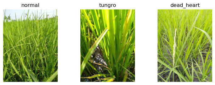
In this section we’ll be experimenting with a few different architectures and image processing approaches (item and batch transforms). In order to make this easier, we’ll put our modeling steps together into a little function which we can pass the architecture, item transforms, and batch transforms to:
def train(arch, item, batch, epochs=5):
    dls = ImageDataLoaders.from_folder(trn_path, seed=42, valid_pct=0.2, item_tfms=item, batch_tfms=batch)
    learn = vision_learner(dls, arch, metrics=error_rate)
    learn.fine_tune(epochs, 0.01)
    return learn
Our item_tfms already resize our images to small sizes, so this shouldn’t impact the accuracy of our models much, if at all. Let’s re-run our resnet26d to test.
learn = train('resnet26d', item=Resize(192),
              batch=aug_transforms(size=128, min_scale=0.75))
/home/stephen137/mambaforge/lib/python3.10/site-packages/torch/amp/autocast_mode.py:198: UserWarning: User provided device_type of 'cuda', but CUDA is not available. Disabling
warnings.warn('User provided device_type of \'cuda\', but CUDA is not available. Disabling')
/home/stephen137/mambaforge/lib/python3.10/site-packages/torch/cuda/amp/grad_scaler.py:115: UserWarning: torch.cuda.amp.GradScaler is enabled, but CUDA is not available. Disabling.
warnings.warn("torch.cuda.amp.GradScaler is enabled, but CUDA is not available. Disabling.")| epoch | train_loss | valid_loss | error_rate | time |
|---|---|---|---|---|
| 0 | 1.915986 | 1.551140 | 0.477174 | 03:13 |
| epoch | train_loss | valid_loss | error_rate | time |
|---|---|---|---|---|
| 0 | 1.242299 | 1.098648 | 0.353676 | 04:09 |
| 1 | 0.969338 | 0.703203 | 0.231619 | 04:05 |
| 2 | 0.744738 | 0.554062 | 0.181643 | 04:04 |
| 3 | 0.532851 | 0.422054 | 0.135031 | 04:15 |
| 4 | 0.423329 | 0.404017 | 0.123979 | 04:10 |
That’s a big improvement in speed, and the accuracy looks fine.
PyTorch Image Models (timm)
PyTorch Image Models (timm) is a wonderful library by Ross Wightman which provides state-of-the-art pre-trained computer vision models. It’s like Hugging Face Transformers, but for computer vision instead of NLP (and it’s not restricted to transformers-based models)!
Ross regularly benchmarks new models as they are added to timm, and puts the results in a CSV in the project’s GitHub repo. To analyse the data, we’ll first clone the repo:
! git clone --depth 1 https://github.com/rwightman/pytorch-image-models.git
%cd pytorch-image-models/results
Cloning into 'pytorch-image-models'...
remote: Enumerating objects: 532, done.
remote: Counting objects: 100% (532/532), done.
remote: Compressing objects: 100% (367/367), done.
remote: Total 532 (delta 222), reused 340 (delta 156), pack-reused 0
Receiving objects: 100% (532/532), 1.30 MiB | 1.21 MiB/s, done.
Resolving deltas: 100% (222/222), done.
/home/stephen137/Kaggle_Comp/pytorch-image-models/resultsUsing Pandas, we can read the two CSV files we need, and merge them together:
import pandas as pd
df_results = pd.read_csv('results-imagenet.csv')
We’ll also add a “family” column that will allow us to group architectures into categories with similar characteristics. Ross told Jeremy Howard which models he’s found the most usable in practice, so we’ll limit the charts to just look at these. (Also include is VGG, not because it’s good, but as a comparison to show how far things have come in the last few years.)
def get_data(part, col):
    df = pd.read_csv(f'benchmark-{part}-amp-nhwc-pt111-cu113-rtx3090.csv').merge(df_results, on='model')
    df['secs'] = 1. / df[col]
    df['family'] = df.model.str.extract('^([a-z]+?(?:v2)?)(?:\d|_|$)')
    df = df[~df.model.str.endswith('gn')]
    df.loc[df.model.str.contains('in22'),'family'] = df.loc[df.model.str.contains('in22'),'family'] + '_in22'
    df.loc[df.model.str.contains('resnet.*d'),'family'] = df.loc[df.model.str.contains('resnet.*d'),'family'] + 'd'
    return df[df.family.str.contains('^re[sg]netd?|beit|convnext|levit|efficient|vit|vgg|swin')]
df = get_data('infer', 'infer_samples_per_sec')Inference results
Here’s the results for inference performance (see the last section for training performance). In this chart:
- the x axis shows how many seconds it takes to process one image (note: it’s a log scale)
- the y axis is the accuracy on Imagenet
- the size of each bubble is proportional to the size of images used in testing
- the color shows what “family” the architecture is from.
Hover your mouse over a marker to see details about the model. Double-click in the legend to display just one family. Single-click in the legend to show or hide a family.
Note: on my screen, Kaggle cuts off the family selector and some plotly functionality – to see the whole thing, collapse the table of contents on the right by clicking the little arrow to the right of “Contents”.
import plotly.express as px
w,h = 1000,800

def show_all(df, title, size):
    return px.scatter(df, width=w, height=h, size=df[size]**2, title=title,
        x='secs',  y='top1', log_x=True, color='family', hover_name='model', hover_data=[size])
show_all(df, 'Inference', 'infer_img_size')I noticed that the GPU usage bar in Kaggle was still nearly empty, so we’re still CPU bound. That means we should be able to use a more capable model with little if any speed impact. convnext_small tops the performance/accuracy tradeoff score there, so let’s give it a go!
ConvNeXT
The ConvNeXT model was proposed in A ConvNet for the 2020s by Zhuang Liu, Hanzi Mao, Chao-Yuan Wu, Christoph Feichtenhofer, Trevor Darrell, Saining Xie. ConvNeXT is a pure convolutional model (ConvNet), inspired by the design of Vision Transformers, that claims to outperform them.
The abstract from the paper is the following:
The “Roaring 20s” of visual recognition began with the introduction of Vision Transformers (ViTs), which quickly superseded ConvNets as the state-of-the-art image classification model. A vanilla ViT, on the other hand, faces difficulties when applied to general computer vision tasks such as object detection and semantic segmentation. It is the hierarchical Transformers (e.g., Swin Transformers) that reintroduced several ConvNet priors, making Transformers practically viable as a generic vision backbone and demonstrating remarkable performance on a wide variety of vision tasks. However, the effectiveness of such hybrid approaches is still largely credited to the intrinsic superiority of Transformers, rather than the inherent inductive biases of convolutions. In this work, we reexamine the design spaces and test the limits of what a pure ConvNet can achieve. We gradually “modernize” a standard ResNet toward the design of a vision Transformer, and discover several key components that contribute to the performance difference along the way. The outcome of this exploration is a family of pure ConvNet models dubbed ConvNeXt. Constructed entirely from standard ConvNet modules, ConvNeXts compete favorably with Transformers in terms of accuracy and scalability, achieving 87.8% ImageNet top-1 accuracy and outperforming Swin Transformers on COCO detection and ADE20K segmentation, while maintaining the simplicity and efficiency of standard ConvNets.
Let’s take a look at one of them…
# choose our vision model architecture
arch = 'convnext_small_in22k'
# feed chosen model into our learner
learn = train(arch, item=Resize(192, method='squish'),
batch=aug_transforms(size=128, min_scale=0.75))| epoch | train_loss | valid_loss | error_rate | time |
|---|---|---|---|---|
| 0 | 1.288349 | 0.913078 | 0.279673 | 05:54 |
| epoch | train_loss | valid_loss | error_rate | time |
|---|---|---|---|---|
| 0 | 0.646190 | 0.435760 | 0.138395 | 34:20 |
| 1 | 0.492490 | 0.374682 | 0.122057 | 34:16 |
| 2 | 0.316289 | 0.239387 | 0.075444 | 34:23 |
| 3 | 0.200733 | 0.164755 | 0.053340 | 34:13 |
| 4 | 0.134689 | 0.158538 | 0.050937 | 34:10 |
# create our test set
tst_files = get_image_files(path/'test_images').sorted()
tst_dl = learn.dls.test_dl(tst_files)
# grab our predictions
probs,_,idxs = learn.get_preds(dl=tst_dl, with_decoded=True)
idxsTensorBase([7, 8, 3, ..., 8, 1, 5])# grab disease names from vocab
dls.vocab['bacterial_leaf_blight', 'bacterial_leaf_streak', 'bacterial_panicle_blight', 'blast', 'brown_spot', 'dead_heart', 'downy_mildew', 'hispa', 'normal', 'tungro']# map disease names to indexes
mapping = dict(enumerate(dls.vocab)) # create a dictionary of the indexes and vocab
results = pd.Series(idxs.numpy(), name="idxs").map(mapping) # looks up the dictionary and returns the indexes, and name of indexes. Passing .map to a dictionary (mapping) is much fasster than passing to a function
results0 hispa
1 normal
2 blast
3 blast
4 blast
...
3464 dead_heart
3465 hispa
3466 normal
3467 bacterial_leaf_streak
3468 dead_heart
Name: idxs, Length: 3469, dtype: object# lets's have a look at the sample Kaggle submisison file
ss = pd.read_csv(path/'sample_submission.csv')
ss| image_id | label | |
|---|---|---|
| 0 | 200001.jpg | NaN |
| 1 | 200002.jpg | NaN |
| 2 | 200003.jpg | NaN |
| 3 | 200004.jpg | NaN |
| 4 | 200005.jpg | NaN |
| ... | ... | ... |
| 3464 | 203465.jpg | NaN |
| 3465 | 203466.jpg | NaN |
| 3466 | 203467.jpg | NaN |
| 3467 | 203468.jpg | NaN |
| 3468 | 203469.jpg | NaN |
3469 rows × 2 columns
# replace 'label' column with our results
ss['label'] = results
ss.to_csv('subm.csv', index=False)
!head subm.csv
image_id,label
200001.jpg,hispa
200002.jpg,normal
200003.jpg,blast
200004.jpg,blast
200005.jpg,blast
200006.jpg,brown_spot
200007.jpg,dead_heart
200008.jpg,brown_spot
200009.jpg,hispa# function to submit to Kaggle
if not iskaggle:
from kaggle import api
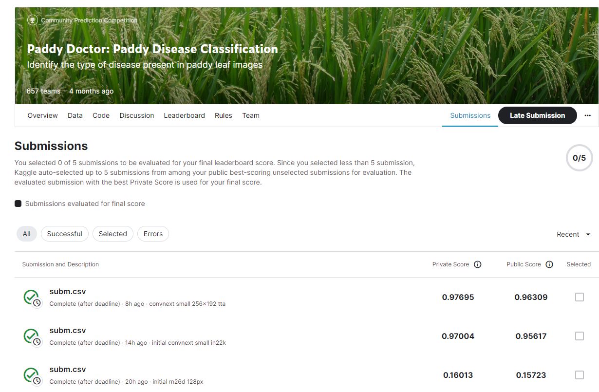
api.competition_submit_cli('subm.csv', 'initial convnext small in22k', comp)100%|██████████████████████████████████████████████████████████████████████████████| 70.5k/70.5k [00:01<00:00, 50.3kB/s]Excellent. This improved model achiveved a public score of 0.95617, comfortably mid table. But, we can do even better:
Pre-processing experiments
So, what shall we try first? One thing which can make a difference is whether we “squish” a rectangular image into a square shape by changing it’s aspect ratio, or randomly crop out a square from it, or whether we add black padding to the edges to make it a square. In the previous version we “squished”.
We can also try padding, which keeps all the original image without transforming it – here’s what that looks like:
# data augmentation using padding
dls = ImageDataLoaders.from_folder(trn_path, valid_pct=0.2, seed=42,
    item_tfms=Resize(192, method=ResizeMethod.Pad, pad_mode=PadMode.Zeros))
dls.show_batch(max_n=3)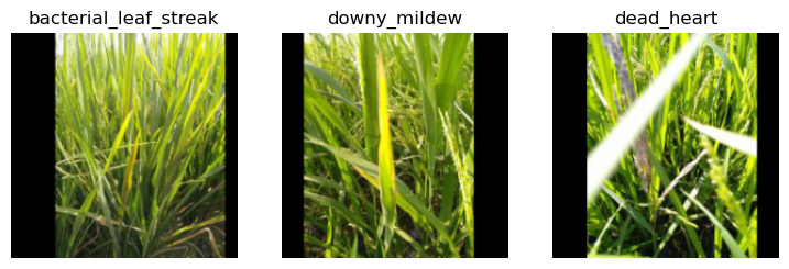
# feed our learner
learn = train(arch, item=Resize((256,192), method=ResizeMethod.Pad, pad_mode=PadMode.Zeros),
batch=aug_transforms(size=(171,128), min_scale=0.75))| epoch | train_loss | valid_loss | error_rate | time |
|---|---|---|---|---|
| 0 | 1.263865 | 0.892569 | 0.281115 | 07:24 |
| epoch | train_loss | valid_loss | error_rate | time |
|---|---|---|---|---|
| 0 | 0.659388 | 0.440261 | 0.138395 | 44:51 |
| 1 | 0.513566 | 0.397354 | 0.131667 | 44:49 |
| 2 | 0.339301 | 0.231382 | 0.067756 | 44:36 |
| 3 | 0.204870 | 0.158647 | 0.047093 | 44:34 |
| 4 | 0.134242 | 0.140719 | 0.044690 | 44:33 |
That’s looking like a pretty good improvement - an error_rate of 0.044690 against 0.050937.
Test time augmentation
To make the predictions even better, we can try test time augmentation (TTA), which our book defines as:
During inference or validation, creating multiple versions of each image, using data augmentation, and then taking the average or maximum of the predictions for each augmented version of the image.
Before trying that out, we’ll first see how to check the predictions and error rate of our model without TTA:
valid = learn.dls.valid
preds,targs = learn.get_preds(dl=valid)
/home/stephen137/mambaforge/lib/python3.10/site-packages/torch/amp/autocast_mode.py:198: UserWarning: User provided device_type of 'cuda', but CUDA is not available. Disabling
warnings.warn('User provided device_type of \'cuda\', but CUDA is not available. Disabling')
/home/stephen137/mambaforge/lib/python3.10/site-packages/torch/cuda/amp/grad_scaler.py:115: UserWarning: torch.cuda.amp.GradScaler is enabled, but CUDA is not available. Disabling.
warnings.warn("torch.cuda.amp.GradScaler is enabled, but CUDA is not available. Disabling.")error_rate(preds, targs)TensorBase(0.0509)That’s the same error rate we saw at the end of training, above, so we know that we’re doing that correctly. Here’s what our data augmentation is doing – if you look carefully, you can see that each image is a bit lighter or darker, sometimes flipped, zoomed, rotated, warped, and/or zoomed:
learn.dls.train.show_batch(max_n=6, unique=True)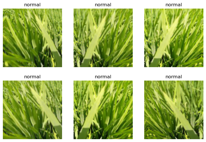
If we call tta() then we’ll get the average of predictions made for multiple different augmented versions of each image, along with the unaugmented original:
tta_preds,_ = learn.tta(dl=valid)Let’s check the error rate of this:
error_rate(tta_preds, targs)TensorBase(0.0375)That’s a huge improvement! We’re now ready to get our Kaggle submission sorted. First, we’ll grab the test set like we did in the last notebook:
tst_files = get_image_files(path/'test_images').sorted()
tst_dl = learn.dls.test_dl(tst_files)
Next, do TTA on that test set:
preds,_ = learn.tta(dl=tst_dl)We need to indices of the largest probability prediction in each row, since that’s the index of the predicted disease. argmax in PyTorch gives us exactly that:
idxs = preds.argmax(dim=1)Now we need to look up those indices in the vocab. Last time we did that using pandas, although since then I realised there’s an even easier way!:
vocab = np.array(learn.dls.vocab)
results = pd.Series(vocab[idxs], name="idxs")
ss = pd.read_csv(path/'sample_submission.csv')
ss['label'] = results
ss.to_csv('subm.csv', index=False)
!head subm.csvimage_id,label
200001.jpg,hispa
200002.jpg,normal
200003.jpg,blast
200004.jpg,blast
200005.jpg,blast
200006.jpg,brown_spot
200007.jpg,dead_heart
200008.jpg,brown_spot
200009.jpg,hispa# submit to Kaggle
if not iskaggle:
from kaggle import api
api.competition_submit_cli('subm.csv', 'convnext small 256x192 tta', comp)100%|██████████████████████████████████████████████████████████████████████████████| 70.4k/70.4k [00:01<00:00, 44.9kB/s]This submission scored 0.96309, improving on our previous submission score of 0.95617.
Iterative approach
It took a long time to train the ConvNeXT model (due to GPU constraints on my machine and also on Paperspace - it’s very rare for there to be any GPU’s available on the free subscription. I’ve since upgraded to ‘Pro’ which costs $8 pm at the time of writing). However you can see the significant improvements made by iterating, and the latest submission of 0.96309 would have been further improved by using larger images and more epochs.
Key takeaways
Most importantly, we have learned the importance of making an early submission to Kaggle, in order to obtain a baseline for rapid improvement through iterating. We’ve also learned some powerful data augmentation techniques, in particular test time augmentation (TTA), how to handle CPU bound environments by resizing images, and discovered the vision model playground that is timm.