Into the Unknown - Efficient Pandas

Introduction

Having code that is clean, readable and has a logical flow is invaluable. I discovered Structured Query Language (SQL) before Python, and as the name suggests, this already pushes you down this structured, logical road. I have only recently started to explore Python, but my experience so far is that the code can quickly become scattered and difficult to follow, particulary during the exploratory data analysis (EDA) phase.

I have just finished actively watching Efficient Pandas by Matt Harrison and decided to share the content via this blog. The video feels like a bit of a breakthrough for me, someone who is just starting out in the world of data science, and hopefully others will also benefit from reading this. Adopting the chaining method covered in this blog, whenever possible, should ensure that your code is cleaner, and reads like a recipe of ordered steps, reducing any potential ambiguities.

Initial set up

# bring in the pandas!
import pandas as pd

# check which version of pandas we're on
pd.__version__

'1.5.0'

# control the pandas display features
pd.options.display.min_rows = 20

Dataset

The dataset we will be exploring is from https://www.fueleconomy.gov/feg/download.shtml which is the official U.S. government source for fuel economy information. The zipped csv file can be downloaded from here but we can just read in the file using pandas:

# read in our dataset
autos = pd.read_csv('https://github.com/mattharrison/datasets/raw/master/data/vehicles.csv.zip')

/tmp/ipykernel_2753/3884461791.py:2: DtypeWarning: Columns (68,70,71,72,73,74,76,79) have mixed types. Specify dtype option on import or set low_memory=False.
  autos = pd.read_csv('https://github.com/mattharrison/datasets/raw/master/data/vehicles.csv.zip')

# Let's take a look
autos

	barrels08	barrelsA08	charge120	charge240	city08	city08U	cityA08	cityA08U	cityCD	cityE	...	mfrCode	c240Dscr	charge240b	c240bDscr	createdOn	modifiedOn	startStop	phevCity	phevHwy	phevComb
0	15.695714	0.0	0.0	0.0	19	0.0	0	0.0	0.0	0.0	...	NaN	NaN	0.0	NaN	Tue Jan 01 00:00:00 EST 2013	Tue Jan 01 00:00:00 EST 2013	NaN	0	0	0
1	29.964545	0.0	0.0	0.0	9	0.0	0	0.0	0.0	0.0	...	NaN	NaN	0.0	NaN	Tue Jan 01 00:00:00 EST 2013	Tue Jan 01 00:00:00 EST 2013	NaN	0	0	0
2	12.207778	0.0	0.0	0.0	23	0.0	0	0.0	0.0	0.0	...	NaN	NaN	0.0	NaN	Tue Jan 01 00:00:00 EST 2013	Tue Jan 01 00:00:00 EST 2013	NaN	0	0	0
3	29.964545	0.0	0.0	0.0	10	0.0	0	0.0	0.0	0.0	...	NaN	NaN	0.0	NaN	Tue Jan 01 00:00:00 EST 2013	Tue Jan 01 00:00:00 EST 2013	NaN	0	0	0
4	17.347895	0.0	0.0	0.0	17	0.0	0	0.0	0.0	0.0	...	NaN	NaN	0.0	NaN	Tue Jan 01 00:00:00 EST 2013	Tue Jan 01 00:00:00 EST 2013	NaN	0	0	0
5	14.982273	0.0	0.0	0.0	21	0.0	0	0.0	0.0	0.0	...	NaN	NaN	0.0	NaN	Tue Jan 01 00:00:00 EST 2013	Tue Jan 01 00:00:00 EST 2013	NaN	0	0	0
6	13.184400	0.0	0.0	0.0	22	0.0	0	0.0	0.0	0.0	...	NaN	NaN	0.0	NaN	Tue Jan 01 00:00:00 EST 2013	Tue Jan 01 00:00:00 EST 2013	NaN	0	0	0
7	13.733750	0.0	0.0	0.0	23	0.0	0	0.0	0.0	0.0	...	NaN	NaN	0.0	NaN	Tue Jan 01 00:00:00 EST 2013	Tue Jan 01 00:00:00 EST 2013	NaN	0	0	0
8	12.677308	0.0	0.0	0.0	23	0.0	0	0.0	0.0	0.0	...	NaN	NaN	0.0	NaN	Tue Jan 01 00:00:00 EST 2013	Tue Jan 01 00:00:00 EST 2013	NaN	0	0	0
9	13.184400	0.0	0.0	0.0	23	0.0	0	0.0	0.0	0.0	...	NaN	NaN	0.0	NaN	Tue Jan 01 00:00:00 EST 2013	Tue Jan 01 00:00:00 EST 2013	NaN	0	0	0
...	...	...	...	...	...	...	...	...	...	...	...	...	...	...	...	...	...	...	...	...	...
41134	16.480500	0.0	0.0	0.0	18	0.0	0	0.0	0.0	0.0	...	NaN	NaN	0.0	NaN	Tue Jan 01 00:00:00 EST 2013	Tue Jan 01 00:00:00 EST 2013	NaN	0	0	0
41135	12.677308	0.0	0.0	0.0	23	0.0	0	0.0	0.0	0.0	...	NaN	NaN	0.0	NaN	Tue Jan 01 00:00:00 EST 2013	Tue Jan 01 00:00:00 EST 2013	NaN	0	0	0
41136	13.733750	0.0	0.0	0.0	21	0.0	0	0.0	0.0	0.0	...	NaN	NaN	0.0	NaN	Tue Jan 01 00:00:00 EST 2013	Tue Jan 01 00:00:00 EST 2013	NaN	0	0	0
41137	11.771786	0.0	0.0	0.0	24	0.0	0	0.0	0.0	0.0	...	NaN	NaN	0.0	NaN	Tue Jan 01 00:00:00 EST 2013	Tue Jan 01 00:00:00 EST 2013	NaN	0	0	0
41138	13.184400	0.0	0.0	0.0	21	0.0	0	0.0	0.0	0.0	...	NaN	NaN	0.0	NaN	Tue Jan 01 00:00:00 EST 2013	Tue Jan 01 00:00:00 EST 2013	NaN	0	0	0
41139	14.982273	0.0	0.0	0.0	19	0.0	0	0.0	0.0	0.0	...	NaN	NaN	0.0	NaN	Tue Jan 01 00:00:00 EST 2013	Tue Jan 01 00:00:00 EST 2013	NaN	0	0	0
41140	14.330870	0.0	0.0	0.0	20	0.0	0	0.0	0.0	0.0	...	NaN	NaN	0.0	NaN	Tue Jan 01 00:00:00 EST 2013	Tue Jan 01 00:00:00 EST 2013	NaN	0	0	0
41141	15.695714	0.0	0.0	0.0	18	0.0	0	0.0	0.0	0.0	...	NaN	NaN	0.0	NaN	Tue Jan 01 00:00:00 EST 2013	Tue Jan 01 00:00:00 EST 2013	NaN	0	0	0
41142	15.695714	0.0	0.0	0.0	18	0.0	0	0.0	0.0	0.0	...	NaN	NaN	0.0	NaN	Tue Jan 01 00:00:00 EST 2013	Tue Jan 01 00:00:00 EST 2013	NaN	0	0	0
41143	18.311667	0.0	0.0	0.0	16	0.0	0	0.0	0.0	0.0	...	NaN	NaN	0.0	NaN	Tue Jan 01 00:00:00 EST 2013	Tue Jan 01 00:00:00 EST 2013	NaN	0	0	0

41144 rows × 83 columns

So our dataset includes 41,144 rows and 83 columns - that’s a lot of data! Let’s have a look at the columns:

autos.columns

Index(['barrels08', 'barrelsA08', 'charge120', 'charge240', 'city08',
       'city08U', 'cityA08', 'cityA08U', 'cityCD', 'cityE', 'cityUF', 'co2',
       'co2A', 'co2TailpipeAGpm', 'co2TailpipeGpm', 'comb08', 'comb08U',
       'combA08', 'combA08U', 'combE', 'combinedCD', 'combinedUF', 'cylinders',
       'displ', 'drive', 'engId', 'eng_dscr', 'feScore', 'fuelCost08',
       'fuelCostA08', 'fuelType', 'fuelType1', 'ghgScore', 'ghgScoreA',
       'highway08', 'highway08U', 'highwayA08', 'highwayA08U', 'highwayCD',
       'highwayE', 'highwayUF', 'hlv', 'hpv', 'id', 'lv2', 'lv4', 'make',
       'model', 'mpgData', 'phevBlended', 'pv2', 'pv4', 'range', 'rangeCity',
       'rangeCityA', 'rangeHwy', 'rangeHwyA', 'trany', 'UCity', 'UCityA',
       'UHighway', 'UHighwayA', 'VClass', 'year', 'youSaveSpend', 'guzzler',
       'trans_dscr', 'tCharger', 'sCharger', 'atvType', 'fuelType2', 'rangeA',
       'evMotor', 'mfrCode', 'c240Dscr', 'charge240b', 'c240bDscr',
       'createdOn', 'modifiedOn', 'startStop', 'phevCity', 'phevHwy',
       'phevComb'],
      dtype='object')

Data Types

Let’s concentrate our focus on a subset of the data. Let’s look at 14 of the 83 columns and also find out about the types of data included. Getting the right types will enable analysis and correctness.

# Let's drill down and focus on just 14 of the 83 columns
cols = ['city08','comb08', 'highway08','cylinders', 'displ', 'drive', 'eng_dscr', 'fuelCost08',
      'make', 'model', 'trany', 'range', 'createdOn', 'year']

# Let's see the data types for each column
autos[cols].dtypes

city08          int64
comb08          int64
highway08       int64
cylinders     float64
displ         float64
drive          object
eng_dscr       object
fuelCost08      int64
make           object
model          object
trany          object
range           int64
createdOn      object
year            int64
dtype: object

# Let's see how much memory is being used by column
autos[cols].memory_usage(deep=True)

Index             128
city08         329152
comb08         329152
highway08      329152
cylinders      329152
displ          329152
drive         3028369
eng_dscr      2135693
fuelCost08     329152
make          2606267
model         2813134
trany         2933276
range          329152
createdOn     3497240
year           329152
dtype: int64

# Let's see how much memory is being used in total
autos[cols].memory_usage(deep=True).sum()

19647323

Integers (int)

Integers(int) are numbers without a decimal point. Let’s grab some summary statistics for our integer columns:

# summary stats for integer columns
(autos
 [cols]
 .select_dtypes(int)
 .describe()
)

	city08	comb08	highway08	fuelCost08	range	year
count	41144.000000	41144.000000	41144.000000	41144.000000	41144.000000	41144.000000
mean	18.369045	20.616396	24.504667	2362.335942	0.793506	2001.535266
std	7.905886	7.674535	7.730364	654.981925	13.041592	11.142414
min	6.000000	7.000000	9.000000	500.000000	0.000000	1984.000000
25%	15.000000	17.000000	20.000000	1900.000000	0.000000	1991.000000
50%	17.000000	20.000000	24.000000	2350.000000	0.000000	2002.000000
75%	20.000000	23.000000	28.000000	2700.000000	0.000000	2011.000000
max	150.000000	136.000000	124.000000	7400.000000	370.000000	2020.000000

Chaining

The above code is fine but it can quickly become cluttered and unreadable. A better way is to lean on SQL coding best practice which means that our code reads more like a recipe of ordered steps:

# use chaining to grab summary stats for integer columns
(autos
 [cols]
 .select_dtypes(int)
 .describe()
)

	city08	comb08	highway08	fuelCost08	range	year
count	41144.000000	41144.000000	41144.000000	41144.000000	41144.000000	41144.000000
mean	18.369045	20.616396	24.504667	2362.335942	0.793506	2001.535266
std	7.905886	7.674535	7.730364	654.981925	13.041592	11.142414
min	6.000000	7.000000	9.000000	500.000000	0.000000	1984.000000
25%	15.000000	17.000000	20.000000	1900.000000	0.000000	1991.000000
50%	17.000000	20.000000	24.000000	2350.000000	0.000000	2002.000000
75%	20.000000	23.000000	28.000000	2700.000000	0.000000	2011.000000
max	150.000000	136.000000	124.000000	7400.000000	370.000000	2020.000000

Same result, much more readable code! Chaining is also known as ‘flow programming’. Rather than creating intermediate variables, leverage the fact that most operations return a new object which can be worked on.

Note, if you can’t find a way to chain we can use pandas .pipe. We’ll see how this works later.

Saving Space

import numpy as np

The int columns are currently in int64 format. Let’s try to free up some space by representing our data more memory efficiently. We can use Numpy to help with this:

# Can comb08 column be int8?
np.iinfo(np.int8)

iinfo(min=-128, max=127, dtype=int8)

The range -128 to 127 can be represented as 8 bits. (There are 256 values which in binary form can be represented by 11111111 i.e. 8 bits). We have a maximum value of 136 for the comb08 column so we can’t convert to int8 without losing info. We can however convert the highway08 column to int8. Let’s try int16:

# Can comb08 column be int16?
np.iinfo(np.int16)

iinfo(min=-32768, max=32767, dtype=int16)

All of our data is within this range, so we can go ahead and convert all int64 columns to int16 (and int8 for highway08):

# convert from int64 to int16 and int8 in order to free up some memory
# also obtain summary statistics for integer columns
(autos
 [cols]
 .astype({'city08': 'int16', 'comb08': 'int16', 'highway08': 'int8','fuelCost08':'int16', 'range':'int16', 'year':'int16'}) 
 .select_dtypes(['integer'])
 .describe()
)

	city08	comb08	highway08	fuelCost08	range	year
count	41144.000000	41144.000000	41144.000000	41144.000000	41144.000000	41144.000000
mean	18.369045	20.616396	24.504667	2362.335942	0.793506	2001.535266
std	7.905886	7.674535	7.730364	654.981925	13.041592	11.142414
min	6.000000	7.000000	9.000000	500.000000	0.000000	1984.000000
25%	15.000000	17.000000	20.000000	1900.000000	0.000000	1991.000000
50%	17.000000	20.000000	24.000000	2350.000000	0.000000	2002.000000
75%	20.000000	23.000000	28.000000	2700.000000	0.000000	2011.000000
max	150.000000	136.000000	124.000000	7400.000000	370.000000	2020.000000

Let’s see if we have saved any space by converting:

# check memory usage
(autos
 [cols]
 .astype({'city08': 'int16', 'comb08': 'int16', 'highway08': 'int8','fuelCost08':'int16', 'range':'int16', 'year':'int16'}) 
 .memory_usage(deep=True)
 .sum() # was 19,647,323
)

18124995

So a saving, but not substantial - just under 8%. Let’s see if we can improve on this:

Floats

A floating point (known as a float) number has decimal points even if that decimal point value is 0. For example: 1.13, 2.0, 1234.345. If we have a column that contains both integers and floating point numbers, Pandas will assign the entire column to the float data type so the decimal points are not lost.

# Let's take a look at the columns with a float data type
(autos
 [cols]
 .select_dtypes('float')
)

	cylinders	displ
0	4.0	2.0
1	12.0	4.9
2	4.0	2.2
3	8.0	5.2
4	4.0	2.2
5	4.0	1.8
6	4.0	1.8
7	4.0	1.6
8	4.0	1.6
9	4.0	1.8
...	...	...
41134	4.0	2.1
41135	4.0	1.9
41136	4.0	1.9
41137	4.0	1.9
41138	4.0	1.9
41139	4.0	2.2
41140	4.0	2.2
41141	4.0	2.2
41142	4.0	2.2
41143	4.0	2.2

41144 rows × 2 columns

Cylinders look int like - we would expect the number of cylinders to be an integer, and not a float (decimal).

# summary stats for cylinders
(autos
 .cylinders
 .describe()
)

count    40938.000000
mean         5.717084
std          1.755517
min          2.000000
25%          4.000000
50%          6.000000
75%          6.000000
max         16.000000
Name: cylinders, dtype: float64

Oops, we have missing values - count = 40,938 but we have 41,144 rows.

# Let's count the various values for cylinders
(autos
 .cylinders
 .value_counts(dropna=False)
)

4.0     15938
6.0     14284
8.0      8801
5.0       771
12.0      626
3.0       279
NaN       206
10.0      170
2.0        59
16.0       10
Name: cylinders, dtype: int64

As anticipated, we have missing values (206) represented by NaN

## where are they missing? We can use .query
(autos
 [cols]
 .query('cylinders.isna()')
)

	city08	comb08	highway08	cylinders	displ	drive	eng_dscr	fuelCost08	make	model	trany	range	createdOn	year
7138	81	85	91	NaN	NaN	NaN	NaN	800	Nissan	Altra EV	NaN	90	Tue Jan 01 00:00:00 EST 2013	2000
7139	81	72	64	NaN	NaN	2-Wheel Drive	NaN	900	Toyota	RAV4 EV	NaN	88	Tue Jan 01 00:00:00 EST 2013	2000
8143	81	72	64	NaN	NaN	2-Wheel Drive	NaN	900	Toyota	RAV4 EV	NaN	88	Tue Jan 01 00:00:00 EST 2013	2001
8144	74	65	58	NaN	NaN	NaN	NaN	1000	Ford	Th!nk	NaN	29	Tue Jan 01 00:00:00 EST 2013	2001
8146	45	39	33	NaN	NaN	2-Wheel Drive	NaN	1700	Ford	Explorer USPS Electric	NaN	38	Tue Jan 01 00:00:00 EST 2013	2001
8147	84	75	66	NaN	NaN	NaN	NaN	900	Nissan	Hyper-Mini	NaN	33	Tue Jan 01 00:00:00 EST 2013	2001
9212	87	78	69	NaN	NaN	2-Wheel Drive	NaN	850	Toyota	RAV4 EV	NaN	95	Tue Jan 01 00:00:00 EST 2013	2002
9213	45	39	33	NaN	NaN	2-Wheel Drive	NaN	1700	Ford	Explorer USPS Electric	NaN	38	Tue Jan 01 00:00:00 EST 2013	2002
10329	87	78	69	NaN	NaN	2-Wheel Drive	NaN	850	Toyota	RAV4 EV	NaN	95	Tue Jan 01 00:00:00 EST 2013	2003
21413	22	24	28	NaN	NaN	4-Wheel Drive	NaN	1750	Subaru	RX Turbo	Manual 5-spd	0	Tue Jan 01 00:00:00 EST 2013	1985
...	...	...	...	...	...	...	...	...	...	...	...	...	...	...
34407	73	72	71	NaN	NaN	Front-Wheel Drive	NaN	900	BYD	e6	Automatic (A1)	187	Wed Mar 13 00:00:00 EDT 2019	2019
34408	118	108	97	NaN	NaN	Front-Wheel Drive	NaN	600	Nissan	Leaf (62 kW-hr battery pack)	Automatic (A1)	226	Wed Mar 13 00:00:00 EDT 2019	2019
34409	114	104	94	NaN	NaN	Front-Wheel Drive	NaN	650	Nissan	Leaf SV/SL (62 kW-hr battery pack)	Automatic (A1)	215	Wed Mar 13 00:00:00 EDT 2019	2019
34538	74	74	73	NaN	NaN	All-Wheel Drive	NaN	900	Audi	e-tron	Automatic (A1)	204	Tue Apr 16 00:00:00 EDT 2019	2019
34561	80	76	72	NaN	NaN	4-Wheel Drive	NaN	850	Jaguar	I-Pace	Automatic (A1)	234	Thu May 02 00:00:00 EDT 2019	2020
34563	138	131	124	NaN	NaN	Rear-Wheel Drive	NaN	500	Tesla	Model 3 Standard Range	Automatic (A1)	220	Thu May 02 00:00:00 EDT 2019	2019
34564	140	133	124	NaN	NaN	Rear-Wheel Drive	NaN	500	Tesla	Model 3 Standard Range Plus	Automatic (A1)	240	Thu May 02 00:00:00 EDT 2019	2019
34565	115	111	107	NaN	NaN	All-Wheel Drive	NaN	600	Tesla	Model S Long Range	Automatic (A1)	370	Thu May 02 00:00:00 EDT 2019	2019
34566	104	104	104	NaN	NaN	All-Wheel Drive	NaN	650	Tesla	Model S Performance (19" Wheels)	Automatic (A1)	345	Thu May 02 00:00:00 EDT 2019	2019
34567	98	97	96	NaN	NaN	All-Wheel Drive	NaN	700	Tesla	Model S Performance (21" Wheels)	Automatic (A1)	325	Thu May 02 00:00:00 EDT 2019	2019

206 rows × 14 columns

## chaining - add cylinders and displ columns replacing NaN with 0
(autos
 [cols]
 .assign(cylinders=autos.cylinders.fillna(0).astype('int8'),
         displ=autos.displ.fillna(0))
 .astype({'city08': 'int16', 'comb08': 'int16', 'highway08': 'int8','fuelCost08':'int16', 'range':'int16', 'year':'int16'}) 
 .describe()
)

	city08	comb08	highway08	cylinders	displ	fuelCost08	range	year
count	41144.000000	41144.000000	41144.000000	41144.000000	41144.000000	41144.000000	41144.000000	41144.000000
mean	18.369045	20.616396	24.504667	5.688460	3.277904	2362.335942	0.793506	2001.535266
std	7.905886	7.674535	7.730364	1.797009	1.373415	654.981925	13.041592	11.142414
min	6.000000	7.000000	9.000000	0.000000	0.000000	500.000000	0.000000	1984.000000
25%	15.000000	17.000000	20.000000	4.000000	2.200000	1900.000000	0.000000	1991.000000
50%	17.000000	20.000000	24.000000	6.000000	3.000000	2350.000000	0.000000	2002.000000
75%	20.000000	23.000000	28.000000	6.000000	4.300000	2700.000000	0.000000	2011.000000
max	150.000000	136.000000	124.000000	16.000000	8.400000	7400.000000	370.000000	2020.000000

# use this to inspect float sizes
np.finfo(np.float16)

finfo(resolution=0.001, min=-6.55040e+04, max=6.55040e+04, dtype=float16)

## chaining - add cylinders and displ columns replacing NaN with 0
(autos
 [cols]
 .assign(cylinders=autos.cylinders.fillna(0).astype('int8'),
         displ=autos.displ.fillna(0).astype('float16'))
 .astype({'city08': 'int16', 'comb08': 'int16', 'highway08': 'int8','fuelCost08':'int16', 'range':'int16', 'year':'int16'}) 
 )

	city08	comb08	highway08	cylinders	displ	drive	eng_dscr	fuelCost08	make	model	trany	range	createdOn	year
0	19	21	25	4	2.000000	Rear-Wheel Drive	(FFS)	2000	Alfa Romeo	Spider Veloce 2000	Manual 5-spd	0	Tue Jan 01 00:00:00 EST 2013	1985
1	9	11	14	12	4.898438	Rear-Wheel Drive	(GUZZLER)	3850	Ferrari	Testarossa	Manual 5-spd	0	Tue Jan 01 00:00:00 EST 2013	1985
2	23	27	33	4	2.199219	Front-Wheel Drive	(FFS)	1550	Dodge	Charger	Manual 5-spd	0	Tue Jan 01 00:00:00 EST 2013	1985
3	10	11	12	8	5.199219	Rear-Wheel Drive	NaN	3850	Dodge	B150/B250 Wagon 2WD	Automatic 3-spd	0	Tue Jan 01 00:00:00 EST 2013	1985
4	17	19	23	4	2.199219	4-Wheel or All-Wheel Drive	(FFS,TRBO)	2700	Subaru	Legacy AWD Turbo	Manual 5-spd	0	Tue Jan 01 00:00:00 EST 2013	1993
5	21	22	24	4	1.799805	Front-Wheel Drive	(FFS)	1900	Subaru	Loyale	Automatic 3-spd	0	Tue Jan 01 00:00:00 EST 2013	1993
6	22	25	29	4	1.799805	Front-Wheel Drive	(FFS)	1700	Subaru	Loyale	Manual 5-spd	0	Tue Jan 01 00:00:00 EST 2013	1993
7	23	24	26	4	1.599609	Front-Wheel Drive	(FFS)	1750	Toyota	Corolla	Automatic 3-spd	0	Tue Jan 01 00:00:00 EST 2013	1993
8	23	26	31	4	1.599609	Front-Wheel Drive	(FFS)	1600	Toyota	Corolla	Manual 5-spd	0	Tue Jan 01 00:00:00 EST 2013	1993
9	23	25	30	4	1.799805	Front-Wheel Drive	(FFS)	1700	Toyota	Corolla	Automatic 4-spd	0	Tue Jan 01 00:00:00 EST 2013	1993
...	...	...	...	...	...	...	...	...	...	...	...	...	...	...
41134	18	20	24	4	2.099609	Front-Wheel Drive	(FFS)	2100	Saab	900	Manual 5-spd	0	Tue Jan 01 00:00:00 EST 2013	1993
41135	23	26	33	4	1.900391	Front-Wheel Drive	(TBI) (FFS)	1600	Saturn	SL	Automatic 4-spd	0	Tue Jan 01 00:00:00 EST 2013	1993
41136	21	24	30	4	1.900391	Front-Wheel Drive	(MFI) (FFS)	1750	Saturn	SL	Automatic 4-spd	0	Tue Jan 01 00:00:00 EST 2013	1993
41137	24	28	33	4	1.900391	Front-Wheel Drive	(TBI) (FFS)	1500	Saturn	SL	Manual 5-spd	0	Tue Jan 01 00:00:00 EST 2013	1993
41138	21	25	32	4	1.900391	Front-Wheel Drive	(MFI) (FFS)	1700	Saturn	SL	Manual 5-spd	0	Tue Jan 01 00:00:00 EST 2013	1993
41139	19	22	26	4	2.199219	Front-Wheel Drive	(FFS)	1900	Subaru	Legacy	Automatic 4-spd	0	Tue Jan 01 00:00:00 EST 2013	1993
41140	20	23	28	4	2.199219	Front-Wheel Drive	(FFS)	1850	Subaru	Legacy	Manual 5-spd	0	Tue Jan 01 00:00:00 EST 2013	1993
41141	18	21	24	4	2.199219	4-Wheel or All-Wheel Drive	(FFS)	2000	Subaru	Legacy AWD	Automatic 4-spd	0	Tue Jan 01 00:00:00 EST 2013	1993
41142	18	21	24	4	2.199219	4-Wheel or All-Wheel Drive	(FFS)	2000	Subaru	Legacy AWD	Manual 5-spd	0	Tue Jan 01 00:00:00 EST 2013	1993
41143	16	18	21	4	2.199219	4-Wheel or All-Wheel Drive	(FFS,TRBO)	2900	Subaru	Legacy AWD Turbo	Automatic 4-spd	0	Tue Jan 01 00:00:00 EST 2013	1993

41144 rows × 14 columns

# new memory usage
(autos
 #[cols]
 .loc[:,cols]
 .assign(cylinders=autos.cylinders.fillna(0).astype('int8'),
         displ=autos.displ.fillna(0).astype('float16'))
 .astype({'city08': 'int16', 'comb08': 'int16', 'highway08': 'int8','fuelCost08':'int16', 'range':'int16', 'year':'int16'}) 
 .memory_usage(deep=True)
 .sum() # was 19,647,323
)

17590123

A further reduction.

Objects

At the very basic level, Pandas objects can be thought of as enhanced versions of NumPy structured arrays in which the rows and columns are identified with labels rather than simple integer indices.

# let's take a look at our object columns
(autos
 [cols]
 .select_dtypes(object)
)

	drive	eng_dscr	make	model	trany	createdOn
0	Rear-Wheel Drive	(FFS)	Alfa Romeo	Spider Veloce 2000	Manual 5-spd	Tue Jan 01 00:00:00 EST 2013
1	Rear-Wheel Drive	(GUZZLER)	Ferrari	Testarossa	Manual 5-spd	Tue Jan 01 00:00:00 EST 2013
2	Front-Wheel Drive	(FFS)	Dodge	Charger	Manual 5-spd	Tue Jan 01 00:00:00 EST 2013
3	Rear-Wheel Drive	NaN	Dodge	B150/B250 Wagon 2WD	Automatic 3-spd	Tue Jan 01 00:00:00 EST 2013
4	4-Wheel or All-Wheel Drive	(FFS,TRBO)	Subaru	Legacy AWD Turbo	Manual 5-spd	Tue Jan 01 00:00:00 EST 2013
5	Front-Wheel Drive	(FFS)	Subaru	Loyale	Automatic 3-spd	Tue Jan 01 00:00:00 EST 2013
6	Front-Wheel Drive	(FFS)	Subaru	Loyale	Manual 5-spd	Tue Jan 01 00:00:00 EST 2013
7	Front-Wheel Drive	(FFS)	Toyota	Corolla	Automatic 3-spd	Tue Jan 01 00:00:00 EST 2013
8	Front-Wheel Drive	(FFS)	Toyota	Corolla	Manual 5-spd	Tue Jan 01 00:00:00 EST 2013
9	Front-Wheel Drive	(FFS)	Toyota	Corolla	Automatic 4-spd	Tue Jan 01 00:00:00 EST 2013
...	...	...	...	...	...	...
41134	Front-Wheel Drive	(FFS)	Saab	900	Manual 5-spd	Tue Jan 01 00:00:00 EST 2013
41135	Front-Wheel Drive	(TBI) (FFS)	Saturn	SL	Automatic 4-spd	Tue Jan 01 00:00:00 EST 2013
41136	Front-Wheel Drive	(MFI) (FFS)	Saturn	SL	Automatic 4-spd	Tue Jan 01 00:00:00 EST 2013
41137	Front-Wheel Drive	(TBI) (FFS)	Saturn	SL	Manual 5-spd	Tue Jan 01 00:00:00 EST 2013
41138	Front-Wheel Drive	(MFI) (FFS)	Saturn	SL	Manual 5-spd	Tue Jan 01 00:00:00 EST 2013
41139	Front-Wheel Drive	(FFS)	Subaru	Legacy	Automatic 4-spd	Tue Jan 01 00:00:00 EST 2013
41140	Front-Wheel Drive	(FFS)	Subaru	Legacy	Manual 5-spd	Tue Jan 01 00:00:00 EST 2013
41141	4-Wheel or All-Wheel Drive	(FFS)	Subaru	Legacy AWD	Automatic 4-spd	Tue Jan 01 00:00:00 EST 2013
41142	4-Wheel or All-Wheel Drive	(FFS)	Subaru	Legacy AWD	Manual 5-spd	Tue Jan 01 00:00:00 EST 2013
41143	4-Wheel or All-Wheel Drive	(FFS,TRBO)	Subaru	Legacy AWD Turbo	Automatic 4-spd	Tue Jan 01 00:00:00 EST 2013

41144 rows × 6 columns

## drive looks categorical
(autos
 .drive
 .value_counts(dropna=False)
)

Front-Wheel Drive             14236
Rear-Wheel Drive              13831
4-Wheel or All-Wheel Drive     6648
All-Wheel Drive                3015
4-Wheel Drive                  1460
NaN                            1189
2-Wheel Drive                   507
Part-time 4-Wheel Drive         258
Name: drive, dtype: int64

# Where are the missing values NaN ?
(autos
 [cols]
 .query('drive.isna()')
)

	city08	comb08	highway08	cylinders	displ	drive	eng_dscr	fuelCost08	make	model	trany	range	createdOn	year
7138	81	85	91	NaN	NaN	NaN	NaN	800	Nissan	Altra EV	NaN	90	Tue Jan 01 00:00:00 EST 2013	2000
8144	74	65	58	NaN	NaN	NaN	NaN	1000	Ford	Th!nk	NaN	29	Tue Jan 01 00:00:00 EST 2013	2001
8147	84	75	66	NaN	NaN	NaN	NaN	900	Nissan	Hyper-Mini	NaN	33	Tue Jan 01 00:00:00 EST 2013	2001
18217	18	21	25	4.0	2.0	NaN	(FFS)	2000	Alfa Romeo	Spider Veloce 2000	Manual 5-spd	0	Tue Jan 01 00:00:00 EST 2013	1984
18218	20	22	26	4.0	1.5	NaN	(FFS)	1900	Bertone	X1/9	Manual 5-spd	0	Tue Jan 01 00:00:00 EST 2013	1984
18219	13	15	20	8.0	5.7	NaN	(350 V8) (FFS)	2800	Chevrolet	Corvette	Automatic 4-spd	0	Tue Jan 01 00:00:00 EST 2013	1984
18220	13	15	20	8.0	5.7	NaN	(350 V8) (FFS)	2800	Chevrolet	Corvette	Manual 4-spd	0	Tue Jan 01 00:00:00 EST 2013	1984
18221	15	17	20	6.0	3.0	NaN	(FFS,TRBO)	2500	Nissan	300ZX	Automatic 4-spd	0	Tue Jan 01 00:00:00 EST 2013	1984
18222	16	18	20	6.0	3.0	NaN	(FFS)	2350	Nissan	300ZX	Automatic 4-spd	0	Tue Jan 01 00:00:00 EST 2013	1984
18223	16	18	22	6.0	3.0	NaN	(FFS,TRBO)	2350	Nissan	300ZX	Manual 5-spd	0	Tue Jan 01 00:00:00 EST 2013	1984
...	...	...	...	...	...	...	...	...	...	...	...	...	...	...
20063	13	15	19	8.0	5.0	NaN	(FFS) CA model	2800	Mercury	Grand Marquis Wagon	Automatic 4-spd	0	Tue Jan 01 00:00:00 EST 2013	1984
20064	13	15	20	8.0	5.0	NaN	(GM-OLDS) CA model	2800	Oldsmobile	Custom Cruiser Wagon	Automatic 4-spd	0	Tue Jan 01 00:00:00 EST 2013	1984
20065	14	16	19	8.0	5.0	NaN	(GM-CHEV) CA model	2650	Pontiac	Parisienne Wagon	Automatic 4-spd	0	Tue Jan 01 00:00:00 EST 2013	1984
20387	14	14	15	4.0	2.4	NaN	(FFS) CA model	3000	Nissan	Pickup Cab Chassis	Manual 5-spd	0	Tue Jan 01 00:00:00 EST 2013	1984
21129	14	16	21	8.0	3.5	NaN	GUZZLER FFS,TURBO	3250	Lotus	Esprit V8	Manual 5-spd	0	Tue Jan 01 00:00:00 EST 2013	2002
23029	79	85	94	NaN	NaN	NaN	Lead Acid	800	GMC	EV1	Automatic (A1)	55	Tue Jan 01 00:00:00 EST 2013	1999
23030	35	37	39	NaN	NaN	NaN	NiMH	1750	GMC	EV1	Automatic (A1)	105	Tue Jan 01 00:00:00 EST 2013	1999
23032	49	48	46	NaN	NaN	NaN	NaN	1400	Honda	EV Plus	Automatic (A1)	81	Tue Jan 01 00:00:00 EST 2013	1999
23037	49	48	46	NaN	NaN	NaN	NaN	1400	Honda	EV Plus	Automatic (A1)	81	Tue Jan 01 00:00:00 EST 2013	1998
23040	102	98	94	NaN	NaN	NaN	NaN	650	MINI	MiniE	Automatic (A1)	100	Tue Jan 01 00:00:00 EST 2013	2008

1189 rows × 14 columns

# let's look at the drive column, grouped by year
(autos
 [cols]
 .groupby('year')
 .drive
 .nunique()
)

year
1984    3
1985    4
1986    4
1987    3
1988    3
1989    3
1990    3
1991    3
1992    3
1993    3
1994    3
1995    4
1996    3
1997    4
1998    4
1999    4
2000    4
2001    4
2002    4
2003    4
2004    4
2005    4
2006    4
2007    4
2008    3
2009    4
2010    6
2011    5
2012    5
2013    5
2014    5
2015    5
2016    5
2017    5
2018    5
2019    5
2020    5
Name: drive, dtype: int64

# let's convert drive to category, replacing NaN with 'Other using .assign .astype
# and convert make to category, updating .astype dictionary 
# and check our memory usage
(autos
 [cols]
 .assign(cylinders=autos.cylinders.fillna(0).astype('int8'),
         displ=autos.displ.fillna(0).astype('float16'),
         drive=autos.drive.fillna('Other').astype('category'))
 .astype({'city08': 'int16', 'comb08': 'int16', 'highway08': 'int8','fuelCost08':'int16', 'range':'int16', 'year':'int16', 'make': 'category'}) 
 .memory_usage(deep=True)
 .sum() # was 19,647,323
)

12093275

As we can see, converting to category has freed up a lot of space, a reduction from 17590123 - just over 30%

# Let's inspect trany 
# looks like it has two pices of info embedded in the column

(autos
 .trany
 .value_counts(dropna=False)
)

Automatic 4-spd                     11047
Manual 5-spd                         8361
Automatic 3-spd                      3151
Automatic (S6)                       3106
Manual 6-spd                         2757
Automatic 5-spd                      2203
Automatic (S8)                       1665
Automatic 6-spd                      1619
Manual 4-spd                         1483
Automatic (S5)                        833
Automatic (variable gear ratios)      826
Automatic 7-spd                       724
Automatic 8-spd                       433
Automatic (AM-S7)                     424
Automatic (S7)                        327
Automatic 9-spd                       293
Automatic (AM7)                       245
Automatic (S4)                        233
Automatic (AV-S6)                     208
Automatic (A1)                        201
Automatic (AM6)                       151
Automatic (AV-S7)                     139
Automatic (S10)                       124
Automatic (AM-S6)                     116
Manual 7-spd                          114
Automatic (S9)                         86
Manual 3-spd                           77
Automatic (AM-S8)                      60
Automatic (AV-S8)                      47
Automatic 10-spd                       25
Manual 4-spd Doubled                   17
Automatic (AM5)                        14
NaN                                    11
Automatic (AV-S10)                     11
Automatic (AM8)                         6
Automatic (AM-S9)                       3
Automatic (L3)                          2
Automatic (L4)                          2
Name: trany, dtype: int64

11 NaN values

The information from the trany column seems to have two components:

Automatic v Manual
Speed

# add new columns for automatic using .str.contains
# add new column for speeds using .str.extract
# drop exisitng trany column
(autos
 [cols]
 .assign(cylinders=autos.cylinders.fillna(0).astype('int8'),
         displ=autos.displ.fillna(0).astype('float16'),
         drive=autos.drive.fillna('Other').astype('category'),
         automatic=autos.trany.str.contains('Auto'),
         speeds=autos.trany.str.extract(r'(\d)+').fillna('20').astype('int8')
        ) 
 .astype({'city08': 'int16', 'comb08': 'int16', 'highway08': 'int8','fuelCost08':'int16', 'range':'int16', 'year':'int16', 'make': 'category'}) 
 .drop(columns=['trany'])
 .memory_usage(deep=True)
 .sum() # was 19,647,323
)

10631047

Great, another reduction - we have almost halved our original memory usage.

Dates

pandas contains extensive capabilities and features for working with time series data for all domains. Check out the documentation for more info.

We can convert the CreatedOn column from an object to datetime using.

# add createdOn using pd.to_datetime .dt.tz_localize
(autos
 [cols]
 .assign(cylinders=autos.cylinders.fillna(0).astype('int8'),
         displ=autos.displ.fillna(0).astype('float16'),
         drive=autos.drive.fillna('Other').astype('category'),
         automatic=autos.trany.str.contains('Auto'),
         speeds=autos.trany.str.extract(r'(\d)+').fillna('20').astype('int8'),
         createdOn=pd.to_datetime(autos.createdOn).dt.tz_localize('America/New_York')
        ) 
 .astype({'city08': 'int16', 'comb08': 'int16', 'highway08': 'int8','fuelCost08':'int16', 'range':'int16', 'year':'int16', 'make': 'category'}) 
 .drop(columns=['trany'])
 .memory_usage(deep=True)
 .sum() # was 19,647,323
)

/home/stephen137/mambaforge/lib/python3.10/site-packages/dateutil/parser/_parser.py:1207: UnknownTimezoneWarning: tzname EST identified but not understood.  Pass `tzinfos` argument in order to correctly return a timezone-aware datetime.  In a future version, this will raise an exception.
  warnings.warn("tzname {tzname} identified but not understood.  "
/home/stephen137/mambaforge/lib/python3.10/site-packages/dateutil/parser/_parser.py:1207: UnknownTimezoneWarning: tzname EDT identified but not understood.  Pass `tzinfos` argument in order to correctly return a timezone-aware datetime.  In a future version, this will raise an exception.
  warnings.warn("tzname {tzname} identified but not understood.  "

Excellent, we have successfully reduced our memory usage by 62%!

# Pythom doesn't like EST/EDT
(autos
 [cols]
 .createdOn
)

0        Tue Jan 01 00:00:00 EST 2013
1        Tue Jan 01 00:00:00 EST 2013
2        Tue Jan 01 00:00:00 EST 2013
3        Tue Jan 01 00:00:00 EST 2013
4        Tue Jan 01 00:00:00 EST 2013
5        Tue Jan 01 00:00:00 EST 2013
6        Tue Jan 01 00:00:00 EST 2013
7        Tue Jan 01 00:00:00 EST 2013
8        Tue Jan 01 00:00:00 EST 2013
9        Tue Jan 01 00:00:00 EST 2013
                     ...             
41134    Tue Jan 01 00:00:00 EST 2013
41135    Tue Jan 01 00:00:00 EST 2013
41136    Tue Jan 01 00:00:00 EST 2013
41137    Tue Jan 01 00:00:00 EST 2013
41138    Tue Jan 01 00:00:00 EST 2013
41139    Tue Jan 01 00:00:00 EST 2013
41140    Tue Jan 01 00:00:00 EST 2013
41141    Tue Jan 01 00:00:00 EST 2013
41142    Tue Jan 01 00:00:00 EST 2013
41143    Tue Jan 01 00:00:00 EST 2013
Name: createdOn, Length: 41144, dtype: object

# Fix date warnings - move on to eng_dscr
# https://www.fueleconomy.gov/feg/findacarhelp.shtml
(autos
 [cols]
 .assign(cylinders=autos.cylinders.fillna(0).astype('int8'),
         displ=autos.displ.fillna(0).astype('float16'),
         drive=autos.drive.fillna('Other').astype('category'),
         automatic=autos.trany.str.contains('Auto'),
         speeds=autos.trany.str.extract(r'(\d)+').fillna('20').astype('int8'),
         createdOn=pd.to_datetime(autos.createdOn.replace({'EDT': '-04:00', 'EST':'-05:00'}, regex=True))
        ) 
 .astype({'city08': 'int16', 'comb08': 'int16', 'highway08': 'int8','fuelCost08':'int16', 'range':'int16', 'year':'int16', 'make': 'category'}) 
 .drop(columns=['trany'])
 .eng_dscr
 .value_counts(dropna=False)
)

NaN                                 16153
(FFS)                                8827
SIDI                                 5526
(FFS) CA model                        926
(FFS)      (MPFI)                     734
FFV                                   701
(FFS,TRBO)                            666
(350 V8) (FFS)                        411
(GUZZLER)  (FFS)                      366
SOHC                                  354
                                    ...  
B234L/R4 (FFS,TRBO)                     1
GUZZLER V8 FFS,TURBO                    1
4.6M FFS MPFI                           1
CNG FFS                                 1
POLICE FFS MPFI                         1
B308E5 FFS,TURBO                        1
5.4E-R FFS MPFI                         1
V-6 FFS                                 1
(GUZZLER)  (FFS)      (S-CHARGE)        1
R-ENG (FFS,TRBO)                        1
Name: eng_dscr, Length: 558, dtype: int64

As we can see the majority of values within the eng_dscr column are NaN and the other values are very messy. How should we deal with this?

# drop eng_dscr column, and bring in an FFS column (feedback fuel system)
# check update to memory usage

(autos
 [cols]
 .assign(cylinders=autos.cylinders.fillna(0).astype('int8'),
         displ=autos.displ.fillna(0).astype('float16'),
         drive=autos.drive.fillna('Other').astype('category'),
         automatic=autos.trany.str.contains('Auto'),
         speeds=autos.trany.str.extract(r'(\d)+').fillna('20').astype('int8'),
         createdOn=pd.to_datetime(autos.createdOn.replace({'EDT': '-04:00', 'EST':'-05:00'}, regex=True)),
         ffs=autos.eng_dscr.str.contains('FFS')
        ) 
 .astype({'city08': 'int16', 'comb08': 'int16', 'highway08': 'int8','fuelCost08':'int16', 'range':'int16', 'year':'int16', 'make': 'category'}) 
 .drop(columns=['trany','eng_dscr'])
 .memory_usage(deep=True)
 .sum() # was 19,647,323
)

Functions - .apply

Let’s now create a function which brings together all the exploratory data analysis we have performed in one place:

def autos_tweak(autos):
    cols = ['city08','comb08', 'highway08','cylinders', 'displ', 'drive', 'eng_dscr', 'fuelCost08',
      'make', 'model', 'trany', 'range', 'createdOn', 'year']
    return (autos
    [cols]
    .assign(cylinders=autos.cylinders.fillna(0).astype('int8'),
         displ=autos.displ.fillna(0).astype('float16'),
         drive=autos.drive.fillna('Other').astype('category'),
         automatic=autos.trany.str.contains('Auto'),
         speeds=autos.trany.str.extract(r'(\d)+').fillna('20').astype('int8'),
         createdOn=pd.to_datetime(autos.createdOn.replace({'EDT': '-04:00', 'EST':'-05:00'}, regex=True)),
         ffs=autos.eng_dscr.str.contains('FFS')
        ) 
    .astype({'city08': 'int16', 'comb08': 'int16',  'highway08': 'int8','fuelCost08':'int16', 'range':'int16', 'year':'int16', 'make': 'category'}) 
    .drop(columns=['trany','eng_dscr'])
    )

Look how neat and tidy the above code is compared to the following alternative approach:

a1 = autos[cols]
cyls = autos.cylinders.fillna(0)
cyls2 = cyls.astype('int8')
a1['cylinders'] = cyls2
displ = a1.displ
displ2 = displ.fillna(0)
displ3=displ2.astype('float16')
a1.displ=displ3
a1.drive=autos.drive.fillna('Other').astype('category')
a1['automatic'] = autos.trany.str.contains('Auto')
speed=autos.trany.str.extract(r'(\d)+')
speedfill = speed.fillna('20')
speedint = speedfill.astype('int8')
a1['speeds'] = speedint
a1.createdOn=pd.to_datetime(autos.createdOn).dt.tz_localize('America/New_York')
a1.ffs=autos.eng_dscr.str.contains('FFS')
a1['highway08'] = autos.highway08.astype('int8')
a1['city08'] = autos.city08.astype('int8')
a1['comb08'] = autos.comb08.astype('int16')
a1['fuelCost08'] =autos.fuelCost08.astype('int16')
a1['range'] = autos.range.astype('int16')
a1['make'] = autos.make.astype('category')
a3 = a1.drop(columns=['trany','eng_dscr'])

Don’t Mutate

“you are missing the point, inplace rarely actually does something inplace. you are thinking that you are saving memory but you are not.”

jreback - Pandas core dev

https://github.com/pandas-dev/pandas/issues/16529#issuecomment-676518136

in general, no performance benefits
prohibits chaining
SettingWithCopyWarning fun

Try to avoid using .apply (where possible)

def autos_tweak(autos):
    cols = ['city08','comb08', 'highway08','cylinders', 'displ', 'drive', 'eng_dscr', 'fuelCost08',
      'make', 'model', 'trany', 'range', 'createdOn', 'year']
    return (autos
    [cols]
    .assign(cylinders=autos.cylinders.fillna(0).astype('int8'),
         displ=autos.displ.fillna(0).astype('float16'),
         drive=autos.drive.fillna('Other').astype('category'),
         automatic=autos.trany.str.contains('Auto'),
         speeds=autos.trany.str.extract(r'(\d)+').fillna('20').astype('int8'),
         createdOn=pd.to_datetime(autos.createdOn.replace({'EDT': '-04:00', 'EST':'-05:00'}, regex=True)),
         ffs=autos.eng_dscr.str.contains('FFS')
        ) 
    .astype({'city08': 'int16', 'comb08': 'int16',  'highway08': 'int8','fuelCost08':'int16', 'range':'int16', 'year':'int16', 'make': 'category'}) 
    .drop(columns=['trany','eng_dscr'])
    )

autos2 = autos_tweak(autos)

# try to be more Euro-centric
def to_lper100km(val):
    return 235.215 / val

%%timeit
autos2.city08.apply(to_lper100km)

5.3 ms ± 390 µs per loop (mean ± std. dev. of 7 runs, 100 loops each)

4.95 ms (milliseconds) is equivalent to 4,950 μs (microseconds)

There is a lot of computational overhead using this method - the function pulls out each individual entry from the Series, convert it to a Python object, pass the individual entry into the function, and then convert back to a pandas object.

%%timeit
# note that you can't run %%timeit with a leading #comment
# this gives the same results
235.215 / autos2.city08

84.5 µs ± 3.29 µs per loop (mean ± std. dev. of 7 runs, 10,000 loops each)

90.7 μs (microseconds)

This gives the same answer but is more than 50 x faster than using the .apply method, because it is leveraging modern CPU single instruction multiple data (SIMD) architecture - here’s a block of data - do the division on it.

# create a function to return whether the make of the car is US
def is_american(val):
    return val in {'Chevrolet', 'Ford', 'Dodge', 'GMC', 'Tesla'}

%%timeit

# use .apply
autos2.make.apply(is_american)

233 µs ± 6.36 µs per loop (mean ± std. dev. of 7 runs, 1,000 loops each)

245 μs (microseconds)

%%timeit

# use .isin 
autos2.make.isin({'Chevrolet', 'Ford', 'Dodge', 'GMC', 'Tesla'})

448 µs ± 9.32 µs per loop (mean ± std. dev. of 7 runs, 1,000 loops each)

465 μs (microseconds)

%%timeit

# use .astype(str) and then .isin
autos2.make.astype(str).isin({'Chevrolet', 'Ford', 'Dodge', 'GMC', 'Tesla'})

4.91 ms ± 65.2 µs per loop (mean ± std. dev. of 7 runs, 100 loops each)

5.35 ms (milliseconds) is equivalent to 5,350 μs (microseconds)

%%timeit

# use .astype(str) and then .apply
autos2.make.astype(str).apply(is_american)

8.23 ms ± 241 µs per loop (mean ± std. dev. of 7 runs, 100 loops each)

8.93 ms (milliseconds) is equivalent to 8,930 μs (microseconds)

In the case of the categorical column - make:

the .apply method on the function was fastest
the .isin method was next fastest (~ 2 x slower)
third fastest was (~ 22 x slower)
finally the .astype(str).apply method (~36 x slower)

def country(val):
    if val in {'Chevrolet', 'Ford', 'Dodge', 'GMC', 'Tesla'}:
        return 'US'
    # else
    return 'Other'

%%timeit

# use .apply
# Might be OK for strings, since they are not vectorized...
(autos2
 .assign(country=autos2.make.apply(country))
)

2.14 ms ± 66.5 µs per loop (mean ± std. dev. of 7 runs, 100 loops each)

%%timeit 

# use .assign
values = {'Chevrolet', 'Ford', 'Dodge', 'GMC', 'Tesla'}
(autos2
 .assign(country='US')
 .assign(country=lambda df_:df_.country.where(df_.make.isin(values), 'Other'))
)

4.31 ms ± 83 µs per loop (mean ± std. dev. of 7 runs, 100 loops each)

%%timeit 

# using MumPy .select - allows you to specify a list of Booleans, and wherever they hold true [i.e make is Chevrolet, Ford, Dodge...Tesla, you specify the value ['US'] to put into placeholder 
# this method is not available within pandas
(autos2
 .assign(country=np.select([autos2.make.isin({'Chevrolet', 'Ford', 'Dodge', 'GMC', 'Tesla'})],
                           ['US'], 'Other'))
)

3.36 ms ± 145 µs per loop (mean ± std. dev. of 7 runs, 100 loops each)

%%timeit 

# using MumPy .where - allows you to specify a list of Booleans, and wherever they hold true [i.e make is Chevrolet, Ford, Dodge...Tesla, you specify the value ['US'] to put into placeholder 
# this method is not available within pandas
(autos2
 .assign(country=np.where(autos2.make.isin({'Chevrolet', 'Ford', 'Dodge', 'GMC', 'Tesla'}),
                           ['US'], 'Other'))
)

3.38 ms ± 35.2 µs per loop (mean ± std. dev. of 7 runs, 100 loops each)

Key takeaways

if you find yourself using a for loop alarm bells should be ringing!
you could use .apply but still slow
apply where or np.select
the same result can be obtained much faster using list comprehension

Aggregation

It is important as a data science to work with the raw data and get to know the finer details, but ultimately, providing higher level insights are our main goal. This can be obtained by aggregating data. Let’s compare mileage by country by year…

# start off with auto
# group by year
# then grab the mean values
(autos2
 # Year will therefore be our index
 .groupby('year')
 .mean()
)

/tmp/ipykernel_2753/262800323.py:7: FutureWarning: The default value of numeric_only in DataFrameGroupBy.mean is deprecated. In a future version, numeric_only will default to False. Either specify numeric_only or select only columns which should be valid for the function.
  .mean()

	city08	comb08	highway08	cylinders	displ	fuelCost08	range	speeds
year
1984	17.982688	19.881874	23.075356	5.385438	3.165017	2313.543788	0.000000	3.928208
1985	17.878307	19.808348	23.042328	5.375661	3.164080	2334.509112	0.000000	3.924750
1986	17.665289	19.550413	22.699174	5.425620	3.183762	2354.049587	0.000000	3.984298
1987	17.310345	19.228549	22.445068	5.412189	3.173949	2403.648757	0.000000	4.037690
1988	17.333628	19.328319	22.702655	5.461947	3.194899	2387.035398	0.000000	4.129204
1989	17.143972	19.125759	22.465742	5.488291	3.209926	2433.434519	0.000000	4.166522
1990	17.033395	19.000928	22.337662	5.496289	3.217369	2436.178108	0.000000	4.238404
1991	16.848940	18.825972	22.253534	5.598940	3.266809	2490.856890	0.000000	4.301237
1992	16.805531	18.862623	22.439786	5.623550	3.276159	2494.736842	0.000000	4.318466
1993	16.998170	19.104300	22.780421	5.602928	3.248540	2454.620311	0.000000	4.339433
1994	16.918534	19.012220	22.725051	5.704684	3.333190	2461.507128	0.000000	4.332994
1995	16.569804	18.797311	22.671148	5.892451	3.471776	2497.828335	0.000000	4.356774
1996	17.289780	19.584735	23.569211	5.627426	3.234789	2375.032342	0.000000	4.364812
1997	17.135171	19.429134	23.451444	5.666667	3.226933	2405.511811	0.000000	4.402887
1998	17.113300	19.518473	23.546798	5.633005	3.201979	2382.635468	0.229064	4.419951
1999	17.272300	19.611502	23.552817	5.667840	3.188794	2392.194836	0.570423	4.421362
2000	17.221429	19.526190	23.414286	5.713095	3.200517	2429.702381	0.348810	4.508333
2001	17.275521	19.479693	23.328211	5.720088	3.192452	2448.463227	0.261251	4.660812
2002	16.893333	19.168205	23.030769	5.827692	3.264525	2479.794872	0.136410	4.757949
2003	16.780651	19.000958	22.836207	5.942529	3.358259	2525.574713	0.090996	4.911877
2004	16.740642	19.067736	23.064171	5.957219	3.393626	2512.566845	0.000000	4.976827
2005	16.851630	19.193825	23.297599	5.944254	3.399485	2518.610635	0.000000	5.192110
2006	16.626812	18.959239	23.048913	6.100543	3.549294	2539.175725	0.000000	5.315217
2007	16.605684	18.978686	23.083481	6.166075	3.628539	2535.923623	0.000000	5.610124
2008	16.900590	19.276327	23.455771	6.192923	3.637796	2536.436394	0.084246	5.773378
2009	17.334459	19.735642	24.017736	6.122466	3.624839	2427.027027	0.000000	6.043074
2010	18.105500	20.588819	24.947701	5.965735	3.502548	2351.082056	0.000000	6.271416
2011	18.669027	21.011504	25.169912	5.980531	3.521903	2333.982301	0.259292	6.560177
2012	19.362847	21.819444	26.105035	5.910590	3.460015	2289.973958	0.782118	6.706597
2013	20.661318	23.125000	27.504223	5.762669	3.327529	2210.768581	1.255068	6.896959
2014	21.033469	23.531429	27.978776	5.745306	3.289703	2198.040816	1.405714	6.985306
2015	21.445830	24.038971	28.586906	5.635230	3.205085	2148.869836	2.208106	7.035853
2016	22.591918	25.150555	29.606973	5.463550	3.054415	2091.204437	4.546751	7.080032
2017	22.761021	25.249033	29.554524	5.453210	3.026032	2096.558391	4.336427	7.225058
2018	22.564732	25.019345	29.273065	5.438988	2.992239	2103.980655	3.519345	7.017113
2019	23.318147	25.627942	29.664389	5.368261	2.964679	2093.545938	5.565680	7.136674
2020	22.679426	25.267943	29.617225	5.071770	2.644994	2023.444976	2.282297	7.746411

# let's focus on just the comb08 and speeds columns
(autos2
 .groupby('year')
 [['comb08','speeds']]
 .mean()
)

	comb08	speeds
year
1984	19.881874	3.928208
1985	19.808348	3.924750
1986	19.550413	3.984298
1987	19.228549	4.037690
1988	19.328319	4.129204
1989	19.125759	4.166522
1990	19.000928	4.238404
1991	18.825972	4.301237
1992	18.862623	4.318466
1993	19.104300	4.339433
1994	19.012220	4.332994
1995	18.797311	4.356774
1996	19.584735	4.364812
1997	19.429134	4.402887
1998	19.518473	4.419951
1999	19.611502	4.421362
2000	19.526190	4.508333
2001	19.479693	4.660812
2002	19.168205	4.757949
2003	19.000958	4.911877
2004	19.067736	4.976827
2005	19.193825	5.192110
2006	18.959239	5.315217
2007	18.978686	5.610124
2008	19.276327	5.773378
2009	19.735642	6.043074
2010	20.588819	6.271416
2011	21.011504	6.560177
2012	21.819444	6.706597
2013	23.125000	6.896959
2014	23.531429	6.985306
2015	24.038971	7.035853
2016	25.150555	7.080032
2017	25.249033	7.225058
2018	25.019345	7.017113
2019	25.627942	7.136674
2020	25.267943	7.746411

%%timeit

# Watch out for the ordering!!!
# here we are grouping by year
# but then we are taking average of all columns - computationally expensive
# we are only interested in comb08 and speeds
(autos2
 .groupby('year')
 .mean()
 #.median()
 #.quantile(.1)
 #.std()
 [['comb08','speeds']]
)

Visualizations

The pandas library includes a variety of visualization tools which allow us to communicate our findings visually. Note that is very easy to show a variety of different plots quickly, simply by commenting out (#) to leave the desired plot:

# in pandas default plot is a line plot
# with index as the x axis and the selected grouped columns as the lines
(autos2
 .groupby('Time_mins')
  [['comb08','speeds']]
 #.mean()
 #.median()
 #.quantile(.1)
 .std()
 #.var()
 .plot()
)

<AxesSubplot: xlabel='year'>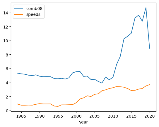

# add country
(autos2
 .assign(country=autos2.make.apply(country))
 # can group by more than one column
 .groupby(['year','country'])
 .mean()
)

/tmp/ipykernel_2753/361744348.py:6: FutureWarning: The default value of numeric_only in DataFrameGroupBy.mean is deprecated. In a future version, numeric_only will default to False. Either specify numeric_only or select only columns which should be valid for the function.
  .mean()

		city08	comb08	highway08	cylinders	displ	fuelCost08	range	speeds
year	country
1984	Other	19.384615	21.417330	24.847038	4.908046	2.690516	2118.125553	0.000000	3.969054
1984	US	16.079232	17.797119	20.669868	6.033613	3.809268	2578.871549	0.000000	3.872749
1985	Other	19.284768	21.373068	24.816777	4.871965	2.636070	2141.997792	0.000000	3.958057
1985	US	16.275472	18.025157	21.020126	5.949686	3.765813	2553.899371	0.000000	3.886792
1986	Other	19.167183	21.213622	24.650155	4.804954	2.536234	2149.148607	0.000000	4.069659
1986	US	15.945035	17.645390	20.464539	6.136525	3.925433	2588.741135	0.000000	3.886525
1987	Other	18.633381	20.710414	24.186876	4.825963	2.583168	2227.318117	0.000000	4.142653
1987	US	15.611722	17.326007	20.208791	6.164835	3.932442	2630.036630	0.000000	3.902930
1988	Other	18.668224	20.814642	24.437695	4.819315	2.531434	2207.476636	0.000000	4.205607
1988	US	15.577869	17.372951	20.420082	6.307377	4.067735	2623.258197	0.000000	4.028689
...	...	...	...	...	...	...	...	...	...
2016	Other	21.903749	24.439716	28.866261	5.493414	2.992272	2127.608916	1.017224	7.296859
2016	US	25.061818	27.701818	32.265455	5.356364	3.277454	1960.545455	17.214545	6.301818
2017	Other	22.423795	24.910521	29.208456	5.431662	2.919041	2114.110128	1.243854	7.474926
2017	US	24.003623	26.496377	30.829710	5.532609	3.420272	2031.884058	15.731884	6.304348
2018	Other	22.310442	24.779868	29.042333	5.396990	2.886801	2121.448730	1.135466	7.391345
2018	US	23.526690	25.925267	30.145907	5.597865	3.391101	2037.900356	12.537367	5.601423
2019	Other	23.084221	25.456922	29.560503	5.315586	2.839671	2093.659245	2.581801	7.545983
2019	US	24.169014	26.250000	30.042254	5.559859	3.419375	2093.133803	16.419014	5.647887
2020	Other	22.579487	25.174359	29.543590	5.148718	2.692823	2050.256410	2.446154	7.743590
2020	US	24.071429	26.571429	30.642857	4.000000	1.978795	1650.000000	0.000000	7.785714

74 rows × 8 columns

# we can go deeper and apply multiple aggregates
# this is loosely equivalent to the sort of thing that a pivot table in Excel might provide

# penultimate row
def second_to_last(ser):
    return ser.iloc[-2]

(autos2
 .assign(country=autos2.make.apply(country))
 .groupby(['year', 'country'])
# we can use .agg to include a list of different aggregation types - we can even call a function
 .agg(['min', 'mean', second_to_last])
)

/tmp/ipykernel_2753/2706922386.py:12: FutureWarning: ['drive', 'make', 'model', 'createdOn'] did not aggregate successfully. If any error is raised this will raise in a future version of pandas. Drop these columns/ops to avoid this warning.
  .agg(['min', 'mean', second_to_last])

		city08			comb08			highway08			cylinders	...	range	automatic			speeds			ffs
		min	mean	second_to_last	min	mean	second_to_last	min	mean	second_to_last	min	...	second_to_last	min	mean	second_to_last	min	mean	second_to_last	min	mean	second_to_last
year	country
1984	Other	7	19.384615	14	8	21.417330	14	9	24.847038	15	2	...	0	False	0.550840	False	3	3.969054	5	False	0.714554	True
1984	US	8	16.079232	15	9	17.797119	17	10	20.669868	19	4	...	0	False	0.521059	False	3	3.872749	4	False	0.638801	NaN
1985	Other	7	19.284768	19	8	21.373068	20	9	24.816777	22	0	...	0	False	0.554084	True	3	3.958057	4	False	0.889160	True
1985	US	8	16.275472	14	10	18.025157	15	10	21.020126	17	3	...	0	False	0.520755	False	3	3.886792	4	False	0.851351	NaN
1986	Other	6	19.167183	10	7	21.213622	11	9	24.650155	12	0	...	0	False	0.520124	False	3	4.069659	4	False	0.934211	NaN
1986	US	9	15.945035	16	10	17.645390	17	11	20.464539	19	3	...	0	False	0.533688	False	3	3.886525	4	False	0.795699	NaN
1987	Other	6	18.633381	12	7	20.710414	12	9	24.186876	12	2	...	0	False	0.516405	True	3	4.142653	4	False	0.949778	True
1987	US	8	15.611722	12	9	17.326007	13	10	20.208791	14	3	...	0	False	0.549451	True	3	3.902930	4	False	0.909457	True
1988	Other	6	18.668224	12	7	20.814642	12	10	24.437695	12	2	...	0	False	0.521807	True	3	4.205607	4	False	0.993681	True
1988	US	8	15.577869	14	9	17.372951	14	10	20.420082	15	3	...	0	False	0.569672	True	3	4.028689	4	False	0.936306	True
...	...	...	...	...	...	...	...	...	...	...	...	...	...	...	...	...	...	...	...	...	...	...
2016	Other	10	21.903749	28	12	24.439716	30	13	28.866261	32	0	...	0	False	0.837893	True	1	7.296859	7	False	0.000000	False
2016	US	11	25.061818	91	12	27.701818	93	16	32.265455	94	0	...	200	False	0.850909	True	1	6.301818	1	False	0.000000	NaN
2017	Other	10	22.423795	21	11	24.910521	24	11	29.208456	28	0	...	0	False	0.848574	True	1	7.474926	7	False	0.000000	False
2017	US	11	24.003623	131	12	26.496377	126	15	30.829710	120	0	...	310	False	0.858696	True	0	6.304348	1	False	0.000000	NaN
2018	Other	9	22.310442	11	11	24.779868	12	11	29.042333	15	0	...	0	False	0.863594	True	0	7.391345	0	False	0.000000	NaN
2018	US	11	23.526690	120	14	25.925267	116	15	30.145907	112	0	...	310	False	0.882562	True	0	5.601423	1	False	0.000000	NaN
2019	Other	9	23.084221	19	11	25.456922	22	14	29.560503	27	0	...	0	False	0.879961	True	0	7.545983	8	False	0.000000	NaN
2019	US	11	24.169014	104	14	26.250000	104	15	30.042254	104	0	...	345	False	0.915493	True	0	5.647887	1	False	0.000000	NaN
2020	Other	13	22.579487	17	15	25.174359	20	18	29.543590	24	0	...	0	False	0.871795	True	0	7.743590	0	False	0.000000	False
2020	US	20	24.071429	21	22	26.571429	24	26	30.642857	28	4	...	0	False	0.857143	True	0	7.785714	0	False	0.000000	False

74 rows × 30 columns

# back to simpler example, adding plots
(autos2
 .assign(country=autos2.make.apply(country))
 # can group by more than one column
 .groupby(['year','country'])
 .mean()
 .plot()
)

/tmp/ipykernel_2753/1855101905.py:6: FutureWarning: The default value of numeric_only in DataFrameGroupBy.mean is deprecated. In a future version, numeric_only will default to False. Either specify numeric_only or select only columns which should be valid for the function.
  .mean()

<AxesSubplot: xlabel='year,country'>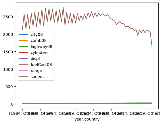

This doesn’t really work as we can see. Let’s see if we can resolve this:

# back to simpler example, adding plots
(autos2
 .assign(country=autos2.make.apply(country))
 # can group by more than one column
 .groupby(['year','country'])
 .mean()
 # rotates or unstacks the innermost index, country
 .unstack()
)

/tmp/ipykernel_2753/1937283994.py:6: FutureWarning: The default value of numeric_only in DataFrameGroupBy.mean is deprecated. In a future version, numeric_only will default to False. Either specify numeric_only or select only columns which should be valid for the function.
  .mean()

	city08		comb08		highway08		cylinders		displ		fuelCost08		range		speeds
country	Other	US	Other	US	Other	US	Other	US	Other	US	Other	US	Other	US	Other	US
year
1984	19.384615	16.079232	21.417330	17.797119	24.847038	20.669868	4.908046	6.033613	2.690516	3.809268	2118.125553	2578.871549	0.000000	0.000000	3.969054	3.872749
1985	19.284768	16.275472	21.373068	18.025157	24.816777	21.020126	4.871965	5.949686	2.636070	3.765813	2141.997792	2553.899371	0.000000	0.000000	3.958057	3.886792
1986	19.167183	15.945035	21.213622	17.645390	24.650155	20.464539	4.804954	6.136525	2.536234	3.925433	2149.148607	2588.741135	0.000000	0.000000	4.069659	3.886525
1987	18.633381	15.611722	20.710414	17.326007	24.186876	20.208791	4.825963	6.164835	2.583168	3.932442	2227.318117	2630.036630	0.000000	0.000000	4.142653	3.902930
1988	18.668224	15.577869	20.814642	17.372951	24.437695	20.420082	4.819315	6.307377	2.531434	4.067735	2207.476636	2623.258197	0.000000	0.000000	4.205607	4.028689
1989	18.533040	15.139831	20.662261	16.908898	24.252570	19.887712	4.879589	6.366525	2.542154	4.173385	2250.000000	2698.093220	0.000000	0.000000	4.264317	4.025424
1990	18.510109	14.850575	20.640747	16.577011	24.267496	19.485057	4.839813	6.466667	2.508090	4.265798	2238.258165	2728.735632	0.000000	0.000000	4.328149	4.105747
1991	18.087943	14.803279	20.174468	16.599532	23.809929	19.683841	5.029787	6.538642	2.610219	4.350876	2348.581560	2725.761124	0.000000	0.000000	4.341844	4.234192
1992	17.915374	14.895631	20.098731	16.735437	23.820874	20.063107	5.145275	6.446602	2.709618	4.251104	2373.272214	2703.762136	0.000000	0.000000	4.356841	4.252427
1993	18.084866	15.007772	20.309760	16.896373	24.172560	20.230570	5.114569	6.497409	2.683870	4.282793	2333.097595	2677.202073	0.000000	0.000000	4.371994	4.279793
1994	18.046474	14.952514	20.264423	16.829609	24.173077	20.201117	5.185897	6.608939	2.713631	4.413091	2326.041667	2697.625698	0.000000	0.000000	4.355769	4.293296
1995	17.678914	14.533724	20.091054	16.422287	24.263578	19.747801	5.444089	6.715543	2.908022	4.506701	2355.191693	2759.677419	0.000000	0.000000	4.380192	4.313783
1996	18.480545	14.926641	20.906615	16.961390	25.093385	20.544402	5.147860	6.579151	2.708768	4.278708	2250.291829	2622.586873	0.000000	0.000000	4.416342	4.262548
1997	18.090909	14.978632	20.509470	16.991453	24.678030	20.683761	5.261364	6.581197	2.786582	4.220544	2319.128788	2600.427350	0.000000	0.000000	4.452652	4.290598
1998	17.925267	15.288000	20.457295	17.408000	24.704626	20.944000	5.275801	6.436000	2.800378	4.104777	2295.373665	2578.800000	0.144128	0.420000	4.485765	4.272000
1999	17.925125	15.709163	20.386023	17.756972	24.577371	21.099602	5.377704	6.362550	2.832181	4.042677	2312.728785	2582.470120	0.251248	1.334661	4.507488	4.215139
2000	17.881849	15.714844	20.301370	17.757812	24.416096	21.128906	5.441781	6.332031	2.859111	3.979351	2385.958904	2529.492188	0.304795	0.449219	4.619863	4.253906
2001	17.941267	15.643939	20.289026	17.496212	24.372488	20.768939	5.479134	6.310606	2.872808	3.975823	2399.536321	2568.371212	0.187017	0.443182	4.761978	4.412879
2002	17.644412	15.083916	20.076923	16.979021	24.207547	20.195804	5.576197	6.433566	2.935398	4.057423	2425.689405	2610.139860	0.137881	0.132867	4.920174	4.367133
2003	17.565101	14.826087	19.953020	16.628763	24.052349	19.806020	5.683221	6.588629	3.032161	4.170778	2480.604027	2637.625418	0.127517	0.000000	5.154362	4.307692
2004	17.426290	14.928571	19.923833	16.805195	24.160934	20.165584	5.729730	6.558442	3.088666	4.199593	2476.719902	2607.305195	0.000000	0.000000	5.229730	4.308442
2005	17.412170	15.196610	19.892078	17.132203	24.189437	20.664407	5.773823	6.447458	3.151592	4.131402	2493.455798	2592.881356	0.000000	0.000000	5.362801	4.688136
2006	17.062575	15.300366	19.509025	17.285714	23.762936	20.875458	5.977136	6.476190	3.345220	4.170487	2527.496992	2574.725275	0.000000	0.000000	5.492178	4.776557
2007	16.996403	15.489726	19.452038	17.626712	23.742206	21.202055	6.044365	6.513699	3.423963	4.212841	2544.664269	2510.958904	0.000000	0.000000	5.864508	4.883562
2008	17.239869	15.770073	19.677985	17.937956	23.983571	21.697080	6.095290	6.518248	3.462049	4.223408	2551.369113	2486.678832	0.109529	0.000000	5.969332	5.120438
2009	17.696803	16.148014	20.186329	18.259928	24.590959	22.140794	5.970232	6.620939	3.402613	4.352489	2433.076075	2407.220217	0.000000	0.000000	6.189636	5.563177
2010	18.325342	17.278970	20.851598	19.600858	25.256849	23.785408	5.897260	6.223176	3.357208	4.048979	2374.429224	2263.304721	0.000000	0.000000	6.378995	5.866953
2011	19.247387	16.817844	21.635308	19.014870	25.855981	22.973978	5.851336	6.394052	3.319702	4.169094	2326.248548	2358.736059	0.340302	0.000000	6.714286	6.066914
2012	19.838052	17.802974	22.339751	20.111524	26.695357	24.167286	5.792752	6.297398	3.268908	4.087332	2282.502831	2314.498141	0.634202	1.267658	6.834655	6.286245
2013	20.982888	19.453815	23.471658	21.823293	27.860963	26.164659	5.658824	6.152610	3.179253	3.884311	2208.288770	2220.080321	0.853476	2.763052	7.033155	6.385542
2014	21.159919	20.506329	23.655870	23.012658	28.088057	27.523207	5.719636	5.852321	3.211738	3.614723	2212.196356	2139.029536	0.859312	3.683544	7.210526	6.046414
2015	21.350000	21.817490	23.935294	24.441065	28.481373	28.996198	5.604902	5.752852	3.101696	3.606063	2164.215686	2089.353612	0.638235	8.296578	7.211765	6.353612
2016	21.903749	25.061818	24.439716	27.701818	28.866261	32.265455	5.493414	5.356364	2.992272	3.277454	2127.608916	1960.545455	1.017224	17.214545	7.296859	6.301818
2017	22.423795	24.003623	24.910521	26.496377	29.208456	30.829710	5.431662	5.532609	2.919041	3.420272	2114.110128	2031.884058	1.243854	15.731884	7.474926	6.304348
2018	22.310442	23.526690	24.779868	25.925267	29.042333	30.145907	5.396990	5.597865	2.886801	3.391101	2121.448730	2037.900356	1.135466	12.537367	7.391345	5.601423
2019	23.084221	24.169014	25.456922	26.250000	29.560503	30.042254	5.315586	5.559859	2.839671	3.419375	2093.659245	2093.133803	2.581801	16.419014	7.545983	5.647887
2020	22.579487	24.071429	25.174359	26.571429	29.543590	30.642857	5.148718	4.000000	2.692823	1.978795	2050.256410	1650.000000	2.446154	0.000000	7.743590	7.785714

# back to simpler example, adding plots
(autos2
 .assign(country=autos2.make.apply(country))
 # can group by more than one column
 .groupby(['year','country'])
 .mean()
 # .std()
 # rotates or unstacks the innermost index, country
 .unstack()
 # focus on city08 column
 .city08
 .plot()
 .legend(bbox_to_anchor=(1,1))
)

/tmp/ipykernel_2753/2308684326.py:6: FutureWarning: The default value of numeric_only in DataFrameGroupBy.mean is deprecated. In a future version, numeric_only will default to False. Either specify numeric_only or select only columns which should be valid for the function.
  .mean()

<matplotlib.legend.Legend at 0x7f2091b75e10>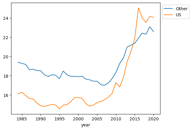

# time series smoothing - rolling average(2)
(autos2
 .assign(country=autos2.make.apply(country))
 # can group by more than one column
 .groupby(['year','country'])
 .mean()
 # .std()
 # rotates or unstacks the innermost index, country
 .unstack()
 # focus on city08 column
 .city08
 # rolling average to smooth time series
 .rolling(2)
 .mean()
 .plot()
 .legend(bbox_to_anchor=(1,1))
)

/tmp/ipykernel_2753/2271732648.py:6: FutureWarning: The default value of numeric_only in DataFrameGroupBy.mean is deprecated. In a future version, numeric_only will default to False. Either specify numeric_only or select only columns which should be valid for the function.
  .mean()

<matplotlib.legend.Legend at 0x7f2091a62ad0>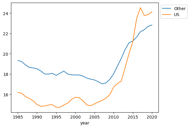

# can we emulate a SQL GROUP BY - HAVING query?
# let's only show grouped values over say 750
def vals_gt(df_, num):
    return df_[df_.gt(num)].dropna()

(autos2
 .assign(country=autos2.make.apply(country))
 # can group by more than one column
 .groupby(['year','country'])
 .count()
 .pipe(vals_gt, 750)
)

		city08	comb08	highway08	cylinders	displ	drive	fuelCost08	make	model	range	createdOn	automatic	speeds	ffs
year	country
1984	Other	1131.0	1131.0	1131.0	1131.0	1131.0	1131.0	1131.0	1131.0	1131.0	1131.0	1131.0	1131.0	1131.0	1065.0
1985	Other	906.0	906.0	906.0	906.0	906.0	906.0	906.0	906.0	906.0	906.0	906.0	906.0	906.0	821.0
2017	Other	1017.0	1017.0	1017.0	1017.0	1017.0	1017.0	1017.0	1017.0	1017.0	1017.0	1017.0	1017.0	1017.0	766.0
2018	Other	1063.0	1063.0	1063.0	1063.0	1063.0	1063.0	1063.0	1063.0	1063.0	1063.0	1063.0	1063.0	1063.0	844.0
2019	Other	1033.0	1033.0	1033.0	1033.0	1033.0	1033.0	1033.0	1033.0	1033.0	1033.0	1033.0	1033.0	1033.0	855.0

Key takeaways

Having code that is clean, readable and has a logical flow is invaluable. Structured Query Language (SQL), as the name suggests, already pushes you down this road. Python, although often referred to as the swiss army knife of programming languages, can quickly beocme scattered and difficult to follow particulary during the exploratory data analysis (EDA) phase. However by adopting the chaining method covered in this blog, your code should ensure that others (as well as yourself!) can follow exactly what is going on.

Although computer memory continues to get cheaper, I think it is good practice to keep track of how much data is being used, and there are some interesting ways covered in this blog as to how we might go about achieving this. e.g. numpy.iinfo. In the same breath, speed is also of the essence, and the handy Python cell magic %%timeit provides an easy way to quantify this. With pandas there is generally a variety of different ways to arrive at the same outcome, but as this blog covers there can be substantial time savings if you know which method to use and when, and which to avoid if possible, in particular the use of .apply.

This blog has been produced in response to the Effective Pandas video presented by Matt Harrison which you can view below. Thanks also to Santiago for the heads up on Twitter.

%%HTML
<iframe width="560" height="315" src="https://www.youtube.com/embed/zgbUk90aQ6A?start=482" title="YouTube video player" frameborder="0" allow="accelerometer; autoplay; clipboard-write; encrypted-media; gyroscope; picture-in-picture" allowfullscreen></iframe>

If the above %%HTML cell magic is unfamiliar to you, then I recommend you watch the excellent video below posted by Corey Shafer. An excellent introduction for anyone starting out with Jupyter NoteBooks.

%%HTML
<iframe width="560" height="315" src="https://www.youtube.com/embed/HW29067qVWk" title="YouTube video player" frameborder="0" allow="accelerometer; autoplay; clipboard-write; encrypted-media; gyroscope; picture-in-picture" allowfullscreen></iframe>