On arrival in Kraków one of the first things to grab my attention was the number of Żabka convenience stores. Those little green frogs seem to be everywhere!
I thought it would be fun to perform a geospatial analysis of the accessibility of these stores. For comparison purposes I chose to also look at Poznań.
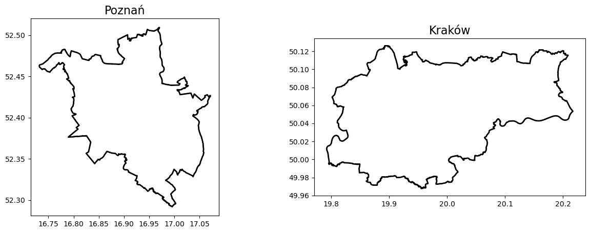
First up, we leverage OSMnx to very quickly grab the administrative boundaries of Kraków and Poznań :
import osmnx as ox # version: 1.0.1import matplotlib.pyplot as plt # version: 3.7.1admin = {}cities = ['Poznań', 'Kraków']f, ax = plt.subplots(1,2, figsize = (15,5))# visualize the admin boundariesfor idx, city inenumerate(cities): admin[city] = ox.geocode_to_gdf(city) admin[city].plot(ax=ax[idx],color='none',edgecolor='k', linewidth =2), ax[idx].set_title(city, fontsize =16)
1.2. Population data
We can create population grids in vector data format for both cities, building on this fine-grained population estimate data source which can be downloaded as a .tif file via WorldPop Hub using the constrained individual countries data set at a resolution of 100m curated in 2020.
import warningswarnings.filterwarnings("ignore")
import rioxarray# rioxarray 0.13.4import xarray as xr # 2022.3.0import datashader as ds # version: 0.15.2import pandas as pdimport numpy as npfrom colorcet import palettefrom datashader import transfer_functions as tf
# # parse the datapoland_file ="pol_ppp_2020_constrained.tif"poland_array = rioxarray.open_rasterio(poland_file, chunks=True, lock=False)
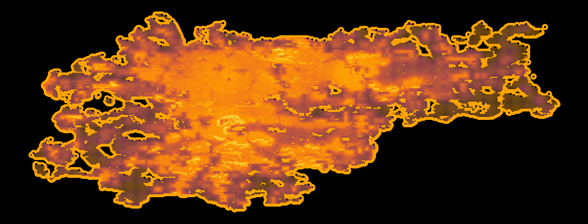
And quickly visualize the population of Poland from this raster file using Matplotlib.
# prepare the datapoland_array = xr.DataArray(poland_array)[0]poland_array = poland_array.where(poland_array >0)poland_array = poland_array.compute()poland_array = np.flip(poland_array, 0)# get the image sizesize =1200asp = poland_array.shape[0] / poland_array.shape[1]# create the data shader canvascvs = ds.Canvas(plot_width=size, plot_height=int(asp*size))raster = cvs.raster(poland_array)# draw the imagecmap = palette["fire"]img = tf.shade(raster, how="eq_hist", cmap=cmap)img = tf.set_background(img, "black")img
We can clearly see the populous cities of (from west to east) Szczecin, Poznań, Wrocław, Gdańsk, Katowice, Łódź, Kraków and Warsaw.
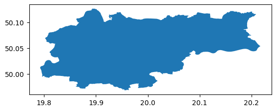
Now that we have visualized Poland let’s look at things at a city level and show you how to transform such raster data into vector format and manipulate it easily with GeoPandas. For this, I access the administrative boundaries of Kraków in a geojson format here. This file contains the boroughs of Kraków, so first, we need to merge them into the city as a whole :
from shapely.ops import cascaded_unionimport geopandas as gpd# Read the GeoJSON filekrakow = gpd.read_file('krakow.geojson')# Perform cascaded union on the geometries and create a new GeoDataFramekrakow = cascaded_union(krakow['geometry'])krakow = gpd.GeoDataFrame(geometry=[krakow])# Plot the resulting GeoDataFramekrakow.plot()
<AxesSubplot: >
Now we can turn the xarray into a Pandas DataFrame, extract the geometry information, and build a GeoPandas GeoDataFrame. One way to do this:
# Specify the output file path and nameoutput_file ='kraków_population_grid.geojson'# Save the GeoDataFrame as a GeoJSON filegdf_krakow.to_file(output_file, driver='GeoJSON')
I performed the same steps for Poznan.
We can make things look nice by creating a custom colormap from the color of 2022, Very Peri.
<class 'geopandas.geodataframe.GeoDataFrame'>
MultiIndex: 355 entries, ('node', 488395425) to ('way', 1056669395)
Columns: 366 entries, name to ways
dtypes: geometry(1), object(365)
memory usage: 1.2+ MB
As you can see our dataframe is of type MultiIndex - we have two different element types - node (which are the Point geometries) and way (which are Polygon geometries). Let’s flatten the dataframe by resetting the index :
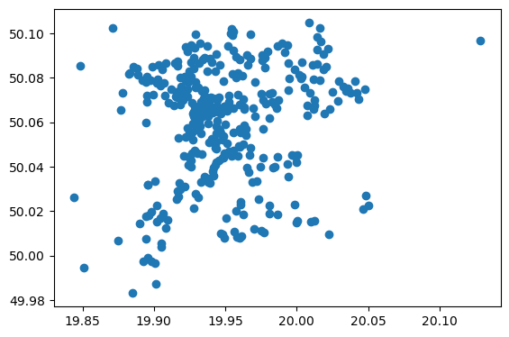
So we now have the locations of 347 stores in Kraków. We can plot them in one line of code :
zabka_krakow.plot()
<AxesSubplot: >
Let’s save our geodatframe to a geoJSON file :
# Specify the output file path and nameoutput_file ='zabka_kraków.geojson'# Save the GeoDataFrame as a GeoJSON filezabka_krakow.to_file(output_file, driver='GeoJSON')
Żabka locations - Poznań
We simply repeat the process for Poznań :
city ='Poznań'
poznan_gdf = ox.geocode_to_gdf(city)poznan_gdf
geometry
bbox_north
bbox_south
bbox_east
bbox_west
place_id
osm_type
osm_id
lat
lon
class
type
place_rank
importance
addresstype
name
display_name
0
POLYGON ((16.73159 52.46375, 16.73162 52.46365...
52.509328
52.291924
17.071707
16.731588
187624076
relation
2456294
52.408266
16.93352
boundary
administrative
12
0.664541
city
Poznań
Poznań, Greater Poland Voivodeship, Poland
shops_poznan = ox.geometries_from_place(
    city,
    tags ={'shop': True}
)
/tmp/ipykernel_552/1581214074.py:1: UserWarning: The `geometries` module and `geometries_from_X` functions have been renamed the `features` module and `features_from_X` functions. Use these instead. The `geometries` module and function names are deprecated and will be removed in a future release.
  shops_poznan = ox.geometries_from_place(
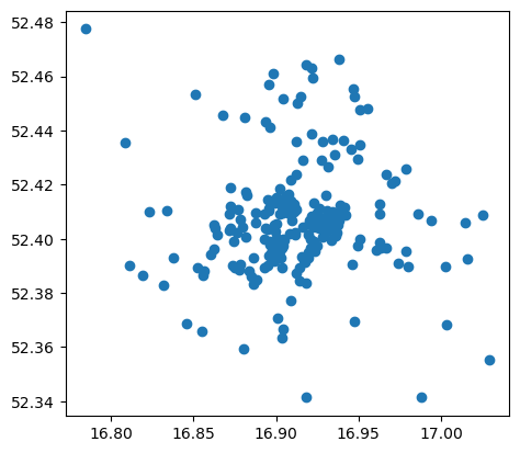
So we have fewer stores in Poznań - 223 against 347 in Kraków - which is not surprising given the comparative populations of the two cities.
zabka_poznan.plot()
<AxesSubplot: >
type(zabka_poznan)
geopandas.geodataframe.GeoDataFrame
Save the file once again to GeoJSON format:
# Specify the output file path and nameoutput_file ='zabka_poznań.geojson'# Save the GeoDataFrame as a GeoJSON filezabka_poznan.to_file(output_file, driver='GeoJSON')
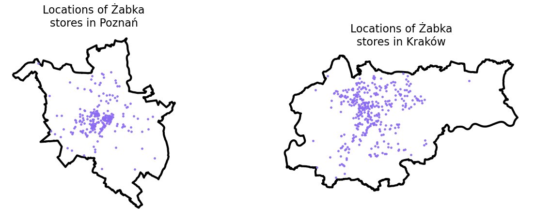
Let’s visualise the distribution of stores in each city side by side:
# parse the data for each citygdf_units= {}gdf_units['Kraków'] = gpd.read_file('zabka_kraków.geojson')gdf_units['Poznań'] = gpd.read_file('zabka_poznań.geojson')for city in cities: gdf_units[city] = gpd.overlay(gdf_units[city], admin[city])# visualize the unitsf, ax = plt.subplots(1,2, figsize = (15,5))for idx, city inenumerate(cities): admin[city].plot(ax=ax[idx],color='none',edgecolor='k', linewidth =3) gdf_units[city].plot( ax=ax[idx], alpha =0.9, color = very_peri, \ markersize =6.0) ax[idx].set_title('Locations of Żabka\nstores in '+ city, \ fontsize =16) ax[idx].axis('off')
2. Accessibilty computation
Referencing this great article written by Nick Jones in 2018 on how to compute pedestrian accessibility:
import os!pip install pandana!pip install osmnetimport pandana # version: 0.6import pandas as pd # version: 1.4.2import numpy as np # version: 1.22.4from shapely.geometry import Point # version: 1.7.1from pandana.loaders import osmdef get_city_accessibility(admin, POIs):# walkability parameters walkingspeed_kmh =5# est mean walking speed walkingspeed_mm = walkingspeed_kmh *1000/60 distance =1609# metres (1 mile)# bounding box as a list of llcrnrlat, llcrnrlng, urcrnrlat, urcrnrlng minx, miny, maxx, maxy = admin.bounds.T[0].to_list() bbox = [miny, minx, maxy, maxx]# setting the input params, going for the nearest POI num_pois =1 num_categories =1 bbox_string ='_'.join([str(x) for x in bbox]) net_filename ='data/network_{}.h5'.format(bbox_string)ifnot os.path.exists('data'): os.makedirs('data')# precomputing nework distancesif os.path.isfile(net_filename):# if a street network file already exists, just load the dataset from that network = pandana.network.Network.from_hdf5(net_filename) method ='loaded from HDF5'else:# otherwise, query the OSM API for the street network within the specified bounding box network = osm.pdna_network_from_bbox(bbox[0], bbox[1], bbox[2], bbox[3]) method ='downloaded from OSM'# identify nodes that are connected to fewer than some threshold of other nodes within a given distance lcn = network.low_connectivity_nodes(impedance=1000, count=10, imp_name='distance') network.save_hdf5(net_filename, rm_nodes=lcn) #remove low-connectivity nodes and save to h5# precomputes the range queries (the reachable nodes within this maximum distance)# so, as long as you use a smaller distance, cached results will be used network.precompute(distance +1)# compute accessibilities on POIs pois = POIs.copy() pois['lon'] = pois.geometry.apply(lambda g: g.x) pois['lat'] = pois.geometry.apply(lambda g: g.y) pois = pois.drop(columns = ['geometry']) network.init_pois(num_categories=num_categories, max_dist=distance, max_pois=num_pois) network.set_pois(category='all', x_col=pois['lon'], y_col=pois['lat'])# searches for the n nearest amenities (of all types) to each node in the network all_access = network.nearest_pois(distance=distance, category='all', num_pois=num_pois)# transform the results into a geodataframe nodes = network.nodes_df nodes_acc = nodes.merge(all_access[[1]], left_index =True, right_index =True).rename(columns = {1 : 'distance'}) nodes_acc['time'] = nodes_acc.distance / walkingspeed_mm xs =list(nodes_acc.x) ys =list(nodes_acc.y) nodes_acc['geometry'] = [Point(xs[i], ys[i]) for i inrange(len(xs))] nodes_acc = gpd.GeoDataFrame(nodes_acc) nodes_acc = gpd.overlay(nodes_acc, admin) nodes_acc[['time', 'geometry']].to_file(city +'_accessibility.geojson', driver ='GeoJSON')return nodes_acc[['time', 'geometry']]accessibilities = {}for city in cities: accessibilities[city] = get_city_accessibility(admin[city], gdf_units[city])
This code block outputs the number of road network nodes in Poznań (105,157) and in Kraków (128,495).
for city in cities:print('Number of road network nodes in '+\ city +': '+str(len(accessibilities[city])))
Number of road network nodes in Poznań: 105157
Number of road network nodes in Kraków: 128495
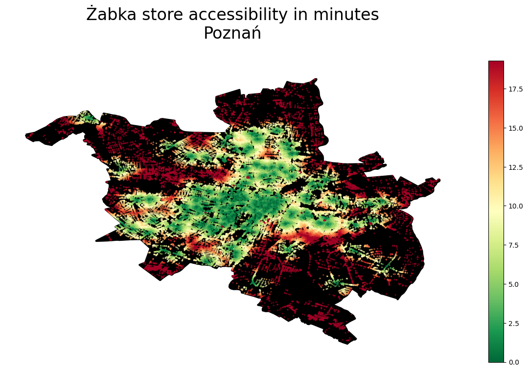
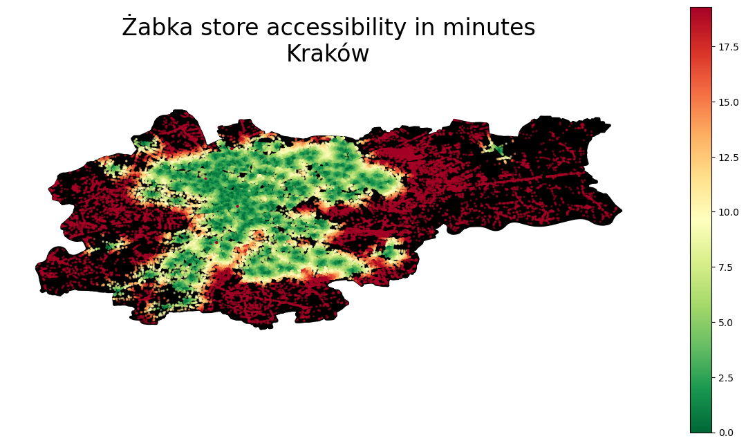
for city in cities: f, ax = plt.subplots(1,1,figsize=(15,8)) admin[city].plot(ax=ax, color ='k', edgecolor ='k', linewidth =3) accessibilities[city].plot(column ='time', cmap ='RdYlGn_r', \ legend =True, ax = ax, markersize =2, alpha =0.5) ax.set_title('Żabka store accessibility in minutes\n'+ city, \ pad =40, fontsize =24) ax.axis('off')
3. Mapping to H3 grid cells
At this point, we have both the population and the accessibility data; we just have to bring them together. The only trick is that their spatial units differ:
Accessibility is measured and attached to each node within the road network of each city
Population data is derived from a raster grid, now described by the POI of each raster grid’s centroid
While rehabilitating the original raster grid may be an option, in the hope of a more pronounced universality let’s map these two types of point data sets into the H3 grid system of Uber. For those who haven’t used it before, for now, its enough to know that it’s an elegant, efficient spatial indexing system using hexagon tiles.
I can’t stop seeing hexagons now!!!
3.1. Creating H3 cells
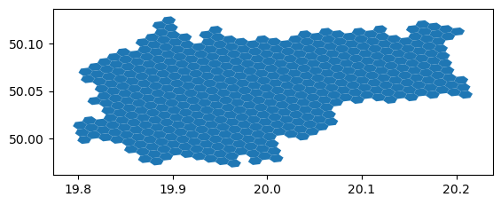
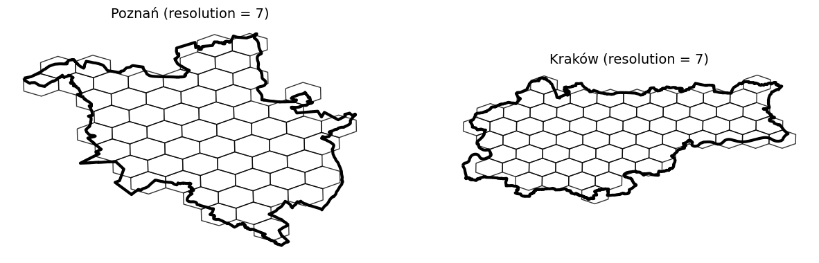
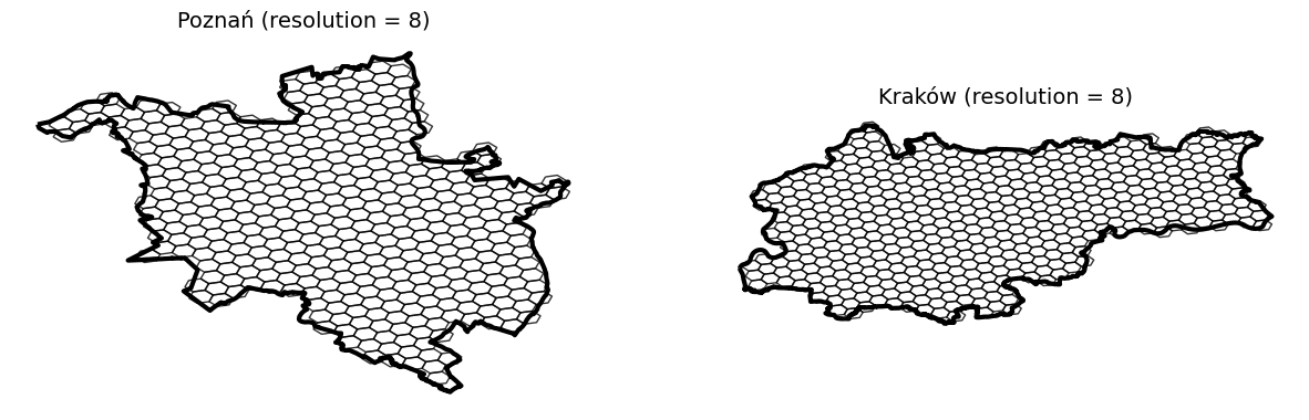
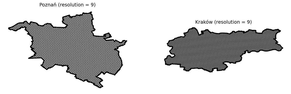
First, put together a function that splits a city into hexagons at any given resolution:
for resolution in [7,8,9]: admin_h3 = {}for city in cities: admin_h3[city] = split_admin_boundary_to_hexagons(admin[city], resolution) f, ax = plt.subplots(1,2, figsize = (15,5))for idx, city inenumerate(cities): admin[city].plot(ax=ax[idx], color ='none', edgecolor ='k', \ linewidth =3) admin_h3[city].plot( ax=ax[idx], alpha =0.8, edgecolor ='k', \ color ='none') ax[idx].set_title(city +' (resolution = '+str(resolution)+')', \ fontsize =14) ax[idx].axis('off')
Let’s stick with resolution 9.
3.2. Map values into h3 cells
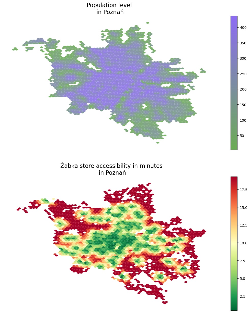
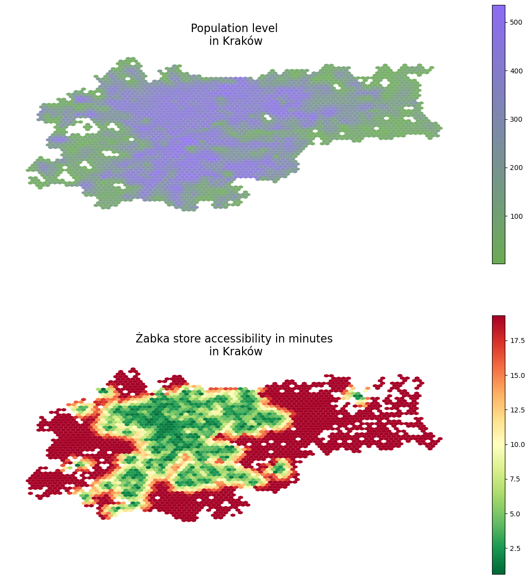
Now, we have both our cities in a hexagon grid format. Next, we shall map the population and accessibility data into the hexagon cells based on which grid cells each point geometry falls into. For this, the sjoin function of GeoPandasa, doing a nice spatial join, is a good choice.
Additionally, as we have more than 100k road network nodes in each city and thousands of population grid centroids, most likely, there will be multiple POIs mapped into each hexagon grid cell. Therefore, aggregation will be needed. As the population is an additive quantity, we will aggregate population levels within the same hexagon by summing them up. However, accessibility is not extensive, so I would instead compute the average store accessibility time for each tile.
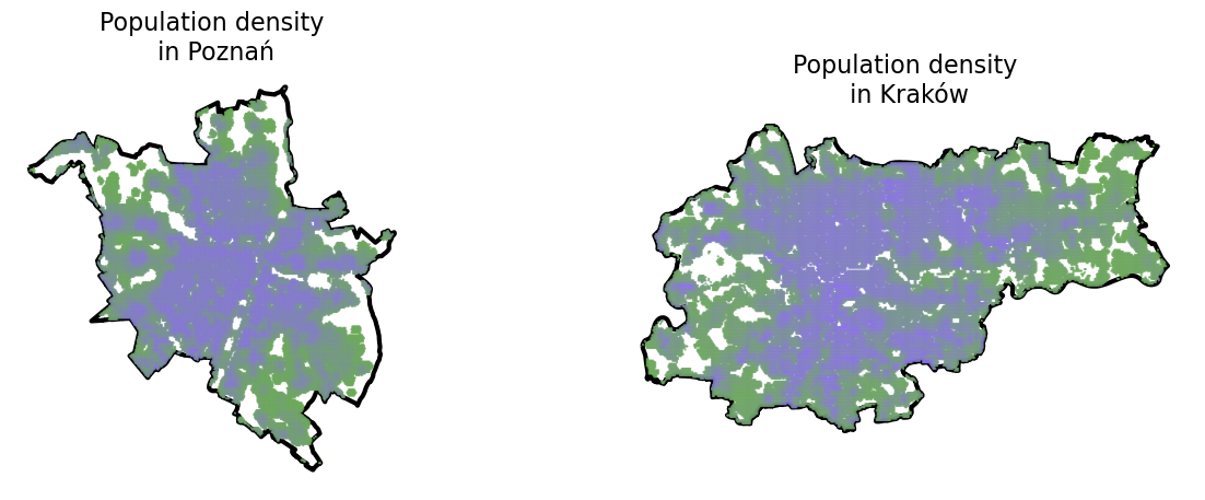
demographics_h3 = {}accessibility_h3 = {}for city in cities:# do the spatial join, aggregate on the population level of each \# hexagon, and then map these population values to the grid ids demographics_dict = gpd.sjoin(admin_h3[city], demographics[city]).groupby(by ='hex_id').sum('population').to_dict()['population'] demographics_h3[city] = admin_h3[city].copy() demographics_h3[city]['population'] = demographics_h3[city].hex_id.map(demographics_dict)# do the spatial join, aggregate on the population level by averaging # accessiblity times within each hexagon, and then map these time score # to the grid ids accessibility_dict = gpd.sjoin(admin_h3[city], accessibilities[city]).groupby(by ='hex_id').mean('time').to_dict()['time'] accessibility_h3[city] = admin_h3[city].copy() accessibility_h3[city]['time'] =\ accessibility_h3[city].hex_id.map(accessibility_dict)# now show the results f, ax = plt.subplots(2,1,figsize = (15,15)) demographics_h3[city].plot(column ='population', legend =True, \ cmap = colormap, ax=ax[0], alpha =0.9, markersize =0.25) accessibility_h3[city].plot(column ='time', cmap ='RdYlGn_r', \ legend =True, ax = ax[1]) ax[0].set_title('Population level\n in '+ city, fontsize =16) ax[1].set_title('Żabka store accessibility in minutes\n in '+ city, \ fontsize =16)for ax_i in ax: ax_i.axis('off')
/tmp/ipykernel_552/223882290.py:9: UserWarning: CRS mismatch between the CRS of left geometries and the CRS of right geometries.
Use `to_crs()` to reproject one of the input geometries to match the CRS of the other.

Left CRS: None
Right CRS: EPSG:4326

  demographics_dict = gpd.sjoin(admin_h3[city], demographics[city]).groupby(by = 'hex_id').sum('population').to_dict()['population']
4. Computing population reach
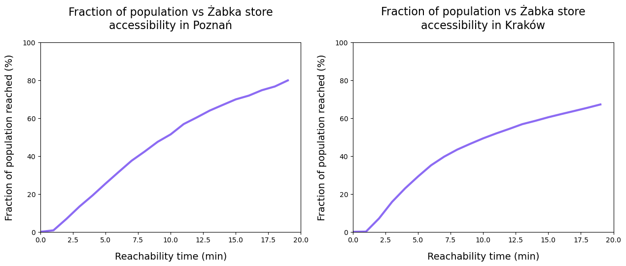
In this final step, we will estimate the fraction of the reachable population from the nearest Żabka store within a certain amount of time. Here, I still build on the relatively fast 15km/h running pace and the 2.5km distance limit.
From the technical perspective, I merge the H3-level population and accessibility time data frames and then do a simple thresholding on the time dimension and a sum on the population dimension.
f, ax = plt.subplots(1,2, figsize = (15,5))for idx, city inenumerate(cities): total_pop = demographics_h3[city].population.sum() merged = demographics_h3[city].merge(accessibility_h3[city].drop(columns =\ ['geometry']), left_on ='hex_id', right_on ='hex_id') time_thresholds =range(20) population_reached = [100*merged[merged.time<limit].population.sum()/total_pop for limit in time_thresholds] ax[idx].plot(time_thresholds, population_reached, linewidth =3, \ color = very_peri) ax[idx].set_xlabel('Reachability time (min)', fontsize =14, \ labelpad =12) ax[idx].set_ylabel('Fraction of population reached (%)', fontsize =14, labelpad =12) ax[idx].set_xlim([0,20]) ax[idx].set_ylim([0,100]) ax[idx].set_title('Fraction of population vs Żabka store\naccessibility in '+ city, pad =20, fontsize =16)
5. Conclusion
When interpreting these results, I would like to emphasize that the store information obtained from Open Street Maps may not be a comprehensive listing of all Żabka stores.
After this disclaimer, what do we see? On the one hand, we see that in both cities, roughly half of the population can get to a store within a 10 minute walk. Extending walking time to 20 minutes results in around 80% access in Poznań, and around 70% access achived in Kraków.
Note that in addition to the caveat of incomplete data, it is important to remember that store accessibility has been calculated based on a walking speed of 5km per hour. This may not be representative of average walking speeds within the cities.
Notwithstanding these reservations, this study provides a solid methodology for combining population data with urban amenity data, to quantify accessibilty. This study can be extended to different cities and amenities across the globe, and the framework is scaleable to different levels of granularity using Uber’s innovative H3 grid system.